AC to DC Formulas: Choose the Circuit Before the Multiplier

An AC voltage does not have one universal DC equivalent. The answer depends on the waveform, the rectifier, any filtering, and the quantity being reported. A calculator that multiplies every AC reading by the same number leaves those decisions hidden. A more useful calculation starts with a circuit model and identifies whether the result is a peak, a complete-cycle average, or an approximate filtered level.

This guide works through three models used by the AC to DC calculator: an ideal unfiltered full-wave rectifier, an ideal unfiltered half-wave rectifier, and a capacitor-filtered bridge estimate. All begin with sinusoidal, single-phase AC RMS voltage at the rectifier input. They solve different problems, so their results should be compared with their assumptions attached.

Start with sinusoidal RMS input

For a sine wave, write the instantaneous input as v = Vm sin θ, where Vm is its positive peak. The mean square of sin θ over a complete cycle is one half. Taking the square root gives Vrms = Vm/√2, or equivalently Vm = √2 × Vrms.

For an input of 12 V RMS, the sine peak is approximately 16.9706 V. That is an input waveform property. It is not automatically the average output of a rectifier, and it does not include diode loss. If the input is a square wave, a distorted waveform, or a peak reading entered as though it were RMS, the calculation has started with the wrong model.

The input location also matters. If a rectifier is connected to a transformer secondary, use the sinusoidal RMS voltage at that secondary under the relevant condition. A primary voltage or an unrelated label elsewhere in the circuit is not interchangeable with the rectifier input.

Ideal full-wave average: about 0.9 times RMS

An ideal full-wave rectifier changes the negative half of the input sine into positive output. Its voltage is Vm|sin θ|. To obtain the average, integrate that waveform over one complete cycle and divide by the cycle length. The area under the absolute sine over 0 to 2π is four, giving Vavg = 2Vm/π.

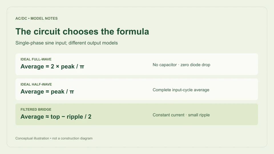
Substituting Vm = √2 Vrms gives Vavg = 2√2 Vrms/π, approximately 0.900316 Vrms. A 12 V RMS input therefore has an ideal full-wave average of about 10.8038 V. The full-wave rectifier calculator uses this complete-cycle average.

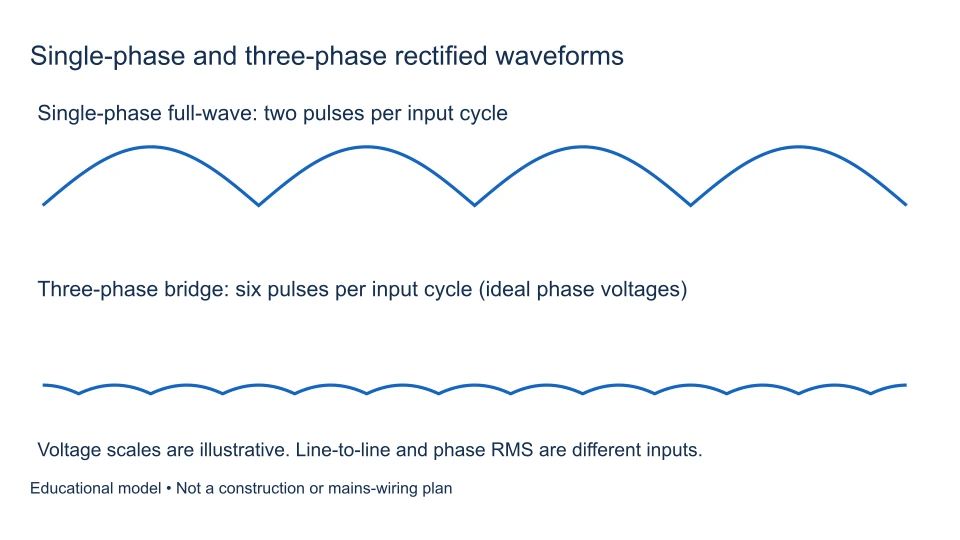
The output is still pulsating. Its peak is approximately 16.9706 V and its valley is zero. Calling the average “DC” describes the nonzero mean component; it does not mean the waveform is flat. This ideal model assumes zero diode drop, no smoothing capacitor, and a resistive load. It is a useful analytical reference, not a prediction of every bridge circuit.

Ideal half-wave average: about 0.45 times RMS

An ideal half-wave rectifier passes one half-cycle and blocks the other. Its complete-cycle average must include the interval during which the output is zero. Integrating the positive half-sine and dividing by the entire 2π cycle gives Vavg = Vm/π.

For sinusoidal RMS input this becomes Vavg = √2 Vrms/π, approximately 0.450158 Vrms. With 12 V RMS input, the ideal average is about 5.4019 V. Its peak remains 16.9706 V because the surviving crest has not changed; there are simply fewer contributing parts of the cycle.

The half-wave calculator reports the complete-cycle average rather than the average of only the conducting half. Confusing those averaging intervals introduces a factor-of-two error. These ideal full-wave and half-wave multipliers agree with the rounded resistive-load factors in Hammond Manufacturing’s rectifier design guide, which also distinguishes rectifier and filter arrangements.

A capacitor-filtered bridge is a different model

A smoothing capacitor changes the shape of the output by storing charge near rectified crests and supplying the load between them. Its average is consequently closer to the available crest than the unfiltered full-wave average, provided the ripple remains small and the charging source behaves approximately as assumed.

The calculator first estimates the available top voltage as Vtop ≈ max(0, √2 Vrms − 2Vf). Vf is the assumed forward drop of one conducting diode. A bridge current path contains two such drops. The default 0.7 V is an illustrative input, not a universal property of silicon diodes.

At 12 V RMS and 0.7 V per diode, the estimated top is 16.9706 − 1.4 = 15.5706 V. That still is not the loaded average. Load current removes charge between crests, causing a voltage decline that must be estimated separately. A zero-load calculation is only a limiting case because leakage and other losses are outside this model.

Derive ripple from charge balance

For approximately constant load current I, charge removed over a time interval Δt is IΔt. For capacitance C, the corresponding voltage change is ΔV = IΔt/C. In a full-wave bridge, charging opportunities occur twice per AC input cycle. Taking the approximate discharge interval as 1/(2f) gives ΔVpp ≈ I/(2fC).

Here f is the AC input frequency in hertz, C is in farads, and I is in amperes. Entered microfarads must be multiplied by 10⁻⁶. Texas Instruments TIDUB95, section 3.1, describes the capacitance and charge relationship and identifies the doubled ripple frequency of a full bridge.

Assuming an approximately linear discharge, its midpoint estimates the average: Vavg ≈ Vtop − ΔVpp/2. The estimated valley is Vvalley ≈ Vtop − ΔVpp. These are deliberately simplified relationships. Charging does not occupy zero time in a real circuit, and a real load may not draw constant current.

Work through the complete 12 V example

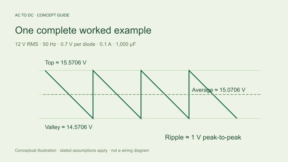
Take 12 V RMS, 50 Hz input, a filtered bridge, 0.7 V per diode, 0.1 A load, and 1,000 µF. Convert capacitance first: 1,000 µF = 0.001 F. The available top is approximately 15.5706 V.

Ripple is 0.1 ÷ (2 × 50 × 0.001), which equals 1 V peak-to-peak. The average estimate is then 15.5706 − 0.5 = 15.0706 V. The estimated valley is 15.5706 − 1 = 14.5706 V, and ripple frequency is 100 Hz.

Those four values answer different questions. The average summarizes the simplified waveform’s mean, the valley describes its lowest estimated point, the peak gives its available top, and ripple describes the difference between top and bottom. None establishes available output current, thermal suitability, or a regulated output specification. A result should include its assumptions rather than being copied as a bare “15 V supply” label.

Understand the approximation guardrail

This site’s filtered model rejects cases where estimated ripple exceeds 20% of the available top voltage. That threshold is a product guardrail chosen to keep large-ripple cases outside a small-ripple approximation. It is not a universal circuit design limit, a component rating, or a promise that every accepted result has a specified error.

If the calculation is rejected, inspect which assumption has become unsuitable. A larger capacitor, lower modeled current, or different operating condition may reduce the estimated ripple, but simply obtaining an accepted number does not validate a circuit. A fuller simulation may be required to represent source impedance, charging pulses, variable load behavior, and diode characteristics.

The model also rejects positive load current when the available sine crest cannot overcome the assumed pair of diode drops. Returning a plausible-looking negative supply voltage would hide the failed assumption. Zero input with zero load can return zero as a mathematical boundary case without implying a real supply’s operating capability.

Avoid common formula substitutions

Do not subtract two fixed diode drops from the ideal full-wave average and assume this exactly models a real bridge. Diodes stop conducting near zero crossings, so the conduction interval changes. A constant subtraction from the entire average is a different approximation and needs its own derivation.

Do not apply the ideal full-wave multiplier to a capacitor-filtered result. Do not use peak-to-peak input voltage as though it were RMS. Do not interpret the same formula as a regulated adapter, inverter, three-phase converter, or switching power supply model. Similar product names do not make their mathematical assumptions equivalent.

For reproducible results, record the input RMS voltage, frequency, selected model, and all active filter settings. State whether the reported output is an ideal waveform average or a filtered estimate. Then read the peak, valley, and ripple together. This makes the calculation useful to another reader and makes discrepancies much easier to investigate.

Check a result without repeating the same mistake

Use a check that is independent of the calculator entry sequence. For an ideal full-wave result, multiply the reported average by π/2 to recover the assumed sine peak, then divide by √2 to recover the input RMS value. For the ideal half-wave average, multiply by π before performing the RMS conversion. This tests whether the averaging convention and the entered waveform description agree.

For the filtered example, add half the reported ripple to the reported average. That should recover the modeled top voltage. Subtract the entire ripple from that top to recover the reported valley. Then add the assumed pair of diode drops and divide by √2 to check the input RMS value. Minor last-digit differences can result from display rounding.

These consistency checks cannot prove that the model matches a physical circuit. They can, however, expose a unit error, the wrong model selection, or a confusion between average and peak before a result is passed to another calculation.

Another useful check is the zero-load limit of the filtered approximation. As the modeled current approaches zero, calculated ripple approaches zero, so average and valley approach the available top. By contrast, the ideal unfiltered full-wave average remains 2Vm/π because its assumed waveform has not changed. Seeing those two different limits helps explain why “no load” is not a reason to mix the models. The output shape and filter assumptions still determine which relationship applies.

Filed under rectifier basics

Topics: AC to DC · formulas · rectifier models