AC to DC calculator worked examples: average, peak, and ripple

A worked example is useful when it shows the assumptions as clearly as the arithmetic. The same AC RMS input can produce different quoted DC quantities because an ideal unfiltered rectifier and a capacitor-filtered bridge do not have the same waveform. Even within one filtered model, the load and capacitor assumptions affect the result.

The examples below use the exact models implemented by the AC to DC calculator. They are hypothetical numerical cases, not measured equipment performance or component recommendations. Each starts by naming the circuit, records the units, and distinguishes peak, average, valley, and peak-to-peak ripple. That makes the results reproducible and prevents a plausible number from being applied to the wrong circuit.

Example one: the default 12 V filtered bridge

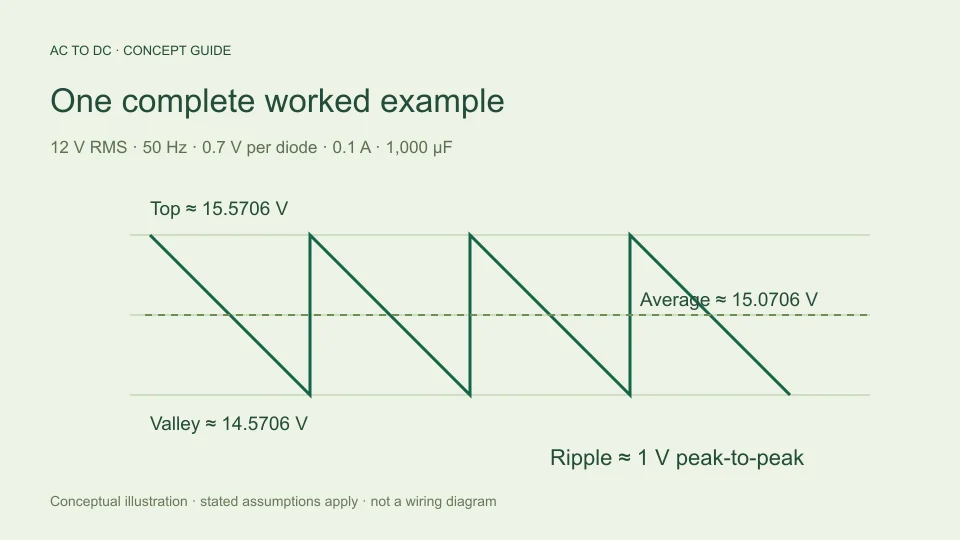
Choose the bridge-plus-capacitor model. Enter 12 V sinusoidal RMS, 50 Hz AC input, an assumed 0.7 V drop per conducting diode, constant 0.1 A load current, and 1,000 µF capacitance.

First calculate the input sine peak: 12 × √2 ≈ 16.970563 V. Two conducting diode drops subtract 1.4 V, leaving an estimated available top of 15.570563 V. Convert capacitance to farads: 1,000 µF = 0.001 F.

Next calculate ripple: 0.1/(2 × 50 × 0.001) = 1 V peak-to-peak. The estimated valley is 15.570563 − 1 = 14.570563 V. The midpoint average is 15.570563 − 0.5 = 15.070563 V. Ripple repetition is 2 × 50 = 100 Hz. These outputs describe an approximate unregulated reservoir waveform, not a regulated supply specification.

Check the default result in reverse

The peak-to-valley difference should equal the displayed ripple: 15.570563 − 14.570563 = 1 V, allowing for rounding. The average should be halfway between those values because the model assumes approximately linear discharge.

Charge balance provides another check. A 0.1 A current over the assumed 0.01-second crest interval removes 0.001 coulombs. Dividing that charge by 0.001 F produces a 1 V change. The same result from a different arrangement of the relationship helps expose a missed unit conversion.

The charge-balance basis and doubled bridge ripple frequency are described in TI TIDUB95, section 3.1. The numerical steps here are independently worked from the stated inputs. They verify the arithmetic of this model, not the accuracy of every omitted circuit effect.

Example two: ideal full-wave without a capacitor

Keep 12 V RMS and 50 Hz, but select ideal full-wave with no filter. Diodes are now assumed lossless and the load is resistive. The capacitor, load-current, and diode-drop controls are irrelevant to this selected model.

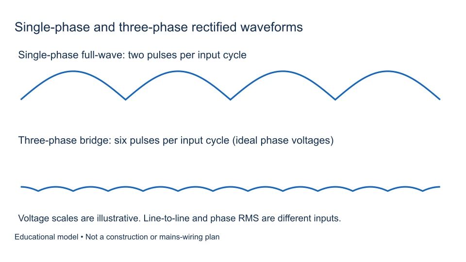
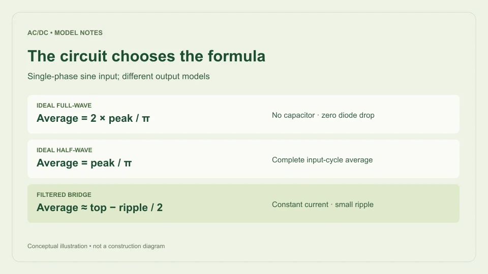
The sine peak remains 16.970563 V. The complete-cycle average of an absolute sine is 2 times its peak divided by π. Therefore average output is 2 × 16.970563/π ≈ 10.803796 V. The waveform’s valley is zero and its peak-to-peak variation is 16.970563 V. It repeats twice per input cycle, giving 100 Hz ripple repetition.

This average is lower than the filtered example because the waveform returns to zero rather than being supported by a storage capacitor. It is not evidence that the calculator has two contradictory conversion factors. It is evidence that the selected circuit model matters.

Example three: ideal half-wave over a complete cycle

Choose ideal half-wave with the same 12 V RMS sine and 50 Hz input. One half-cycle contributes output while the other is blocked. The average is calculated over the entire input period, including the blocked half-cycle.

The average is peak divided by π: 16.970563/π ≈ 5.401898 V. Peak remains 16.970563 V, valley is zero, and the waveform repeats once per AC cycle, giving 50 Hz ripple repetition. The average is half the ideal full-wave result for the same RMS input.

As a scale check, the rounded ideal factors are about 0.45 times RMS for half-wave and 0.90 times RMS for full-wave. Those resistive-load approximations agree with Hammond Manufacturing’s rectifier guide. Use the analytical expressions when checking more digits, rather than treating rounded multipliers as exact constants.

Example four: a 24 V, 60 Hz filtered estimate

Return to the filtered bridge model. Use 24 V RMS, 60 Hz, 0.7 V per diode, 0.2 A load, and 2,200 µF. The sine peak is 24√2 ≈ 33.941125 V. Subtracting 1.4 V gives a top of about 32.541125 V.

Convert 2,200 µF to 0.0022 F. Estimated ripple is 0.2/(2 × 60 × 0.0022), approximately 0.757576 V peak-to-peak. Subtracting this from the top gives a valley of about 31.783550 V. Subtracting half gives an average of about 32.162338 V. Ripple repetition is 120 Hz.

The result is still an approximation under a constant-current load with fixed diode drops and a simplified discharge shape. None of the input values establishes the suitability of a transformer, bridge, or capacitor. The example exercises the arithmetic with a different voltage, frequency, current, and microfarad conversion.

Example five: isolate the frequency change

Use the default filtered settings but change input frequency from 50 Hz to 60 Hz. Hold RMS voltage, assumed diode drop, current, and capacitance fixed. The available top remains approximately 15.570563 V because the model’s top-voltage equation does not contain frequency.

Ripple becomes 0.1/(120 × 0.001) ≈ 0.833333 V. The midpoint average becomes about 15.153896 V, and the valley becomes about 14.737229 V. Ripple repetition changes from 100 Hz to 120 Hz.

This comparison isolates the modeled discharge interval. It does not demonstrate that an actual transformer is suitable for either input frequency or that its real secondary RMS voltage remains unchanged. Holding variables fixed is an analytical choice that should be stated, rather than quietly assumed to describe all equipment behavior.

Example six: the zero-load limiting case

Set the filtered model’s load current to zero while leaving the default voltage, frequency, diode drop, and capacitance. The charge-balance expression then gives zero discharge ripple. Peak, average, and valley all become the same estimated level, about 15.570563 V.

This is a mathematical limiting case. Leakage, measurement loading, and other currents are omitted. The result does not prove that a physical unloaded capacitor will hold a perfectly constant voltage or that an actual diode maintains a 0.7 V drop at vanishing current.

At zero AC input and zero load, the model returns zero rather than a negative capacitor voltage after subtracting diode drops. At insufficient input peak with positive requested load, it rejects the case. That is preferable to displaying a negative supply value that the selected bridge model does not describe.

Example seven: a case outside the small-ripple scope

Take the default filtered settings but reduce capacitance to 100 µF. The charge-balance expression would give ripple 0.1/(100 × 0.0001) = 10 V peak-to-peak. Relative to the available 15.570563 V top, that is about 64%.

The calculator rejects this case because its chosen guardrail is 20% of available peak. It does not publish a midpoint output as though the same small-ripple approximation remained appropriate. The warning calls for a more suitable model or a genuinely different scenario, rather than an arbitrary input change made only to suppress the warning.

The 20% threshold is a product scope decision, not a universal component-design criterion and not a guaranteed percentage-error bound. A case below it can still differ from actual hardware because omitted effects remain omitted. The rejection tells you about this model’s limits.

Check inputs and rounding before comparing results

Negative RMS voltage, nonpositive frequency, unsupported model names, non-finite numbers, and out-of-range physical inputs are rejected. A negative RMS entry is not how input polarity is represented in this model. RMS is a nonnegative magnitude, while the rectifier’s output convention is defined by the circuit.

Display values are rounded to eight significant digits. Carry extra digits during an independent calculation and round only when comparing displayed output. A small last-digit difference caused by formatting is different from a factor-of-two frequency error or a millionfold capacitance-unit error.

The most useful comparison record includes every input and the selected model. “The answer should be 15 V” is difficult to evaluate; a complete input set and a written formula let another reader reproduce the calculation and decide whether the disagreement is mathematical or conceptual.

Decide what the example has actually verified

These examples verify numerical relationships within the stated circuit models. They do not validate transformer regulation, diode temperature behavior, charging-current pulses, capacitor ESR, transient loads, regulator headroom, or component ratings. Those questions require additional evidence and a fuller model.

When reporting a result, use its proper name: ideal waveform average, estimated filtered average, available top, estimated valley, or peak-to-peak ripple. Preserve the assumptions beside the value. This makes the calculator useful as a transparent explanation rather than a source of unexplained multipliers.

For a deeper understanding of the default result, read the capacitor ripple guide and the rectifier formula comparison. They explain why each equation applies where it does and why a different circuit deserves a different calculation.

Prepare an issue report that someone can reproduce

If a result appears wrong, include the input RMS value, selected rectifier mode, input frequency, and every active filtered setting. State the displayed quantity you disagree with and show an independently worked expected value. Include the formula and units rather than only a screenshot of a final number.

For example, a useful report might state that a filtered bridge at 12 V RMS, 50 Hz, 0.1 A, 1,000 µF, and 0.7 V per diode should have 1 V peak-to-peak ripple because the denominator is 0.1. That evidence immediately identifies the model and arithmetic being checked. A report about an ideal unfiltered average would use a different formula and should say so.

Also distinguish a calculation discrepancy from a mismatch with physical equipment. A measurement can differ because its waveform, location, load, or omitted circuit behavior differs from the assumptions. Recording those details helps decide whether the correction belongs in the arithmetic, input interpretation, model explanation, or a more complete analysis of the circuit itself.

Filed under worked examples rectifier basics

Topics: AC to DC examples · bridge calculator · ripple