AC/DC Calc
rectifier basics · worked examples
Capacitor Ripple Explained: What Happens Between Charging Peaks
Derive bridge ripple from charge balance, work through units, and understand where the small-ripple approximation stops being useful.
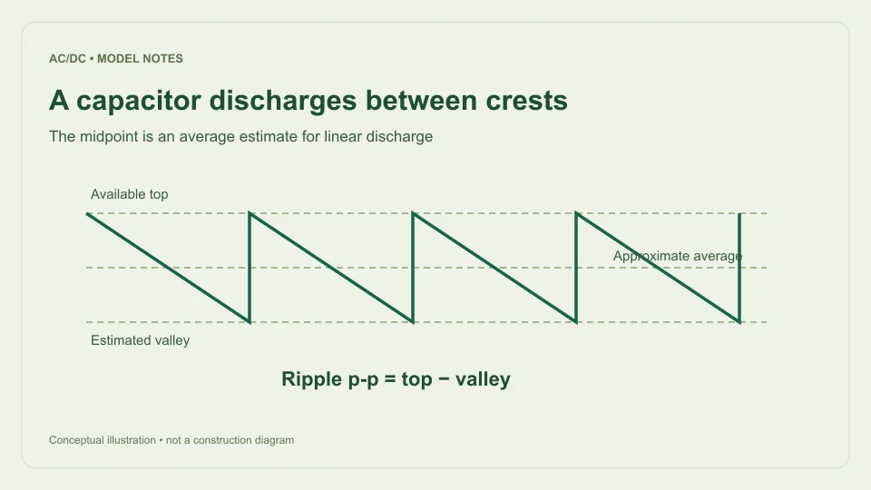
A smoothing capacitor reduces changes in rectifier output, but it does not create a perfectly constant voltage. Between charging crests, the load removes charge from the capacitor and its voltage falls. A useful ripple calculation describes that discharge while being explicit about how it approximates the recharge process.
This guide explains the filtered bridge model used by the AC to DC calculator. It assumes a sinusoidal single-phase input, a bridge rectifier, approximately constant load current, fixed diode forward drop, and small approximately linear ripple. It estimates voltage behavior rather than selecting components or guaranteeing the performance of a physical power supply.
Begin with stored charge
The defining capacitor relationship is Q = CV. If capacitance remains constant, a change in stored charge corresponds to ΔQ = CΔV. Current is the rate of charge flow, so constant current over an interval Δt removes charge IΔt.
Combining those relationships gives ΔV = IΔt/C. The expression has a straightforward interpretation: more current removes more charge, more discharge time allows a larger decline, and more capacitance produces a smaller voltage change for the same lost charge.
The units check the result. An ampere is a coulomb per second, so amperes multiplied by seconds gives coulombs. A farad is a coulomb per volt. Dividing coulombs by farads therefore gives volts. This dimensional check is a useful way to catch a missing frequency factor or a microfarad conversion error before interpreting a numerical answer.
Why a bridge uses twice the input frequency
Full-wave rectification brings both input half-cycles to the same output polarity. A 50 Hz sine has one positive and one negative crest in each 20 ms input cycle. After ideal full-wave rectification, those crests become two positive charging opportunities approximately 10 ms apart.
The simple ripple estimate uses Δt ≈ 1/(2f), where f is the AC input frequency. Substituting this into charge balance gives ΔVpp ≈ I/(2fC). The doubled frequency and capacitor charge relationship are described in Texas Instruments TIDUB95, section 3.1.
The approximation treats the capacitor as if it recharges near each crest and then discharges over nearly the entire interval to the next one. Actual charging takes a finite time. The relationship is most useful when that distinction is modest and the resulting ripple is small relative to the available top voltage.
Use farads in the equation
Capacitors are often described in microfarads, but the equation uses farads. One microfarad is 10⁻⁶ F, so 1,000 µF becomes 0.001 F. Entering 1,000 as the farad value would introduce a factor-of-one-million error.
Current needs the same attention. A load of 100 mA is 0.1 A. Frequency is the original AC input frequency, such as 50 Hz, because the formula already contains the factor of two for a bridge. Entering 100 Hz as the input and then multiplying by two again halves the predicted ripple incorrectly.
A reliable record keeps units attached to every input: 0.1 A, 50 Hz input, and 0.001 F. The calculator labels the user-facing capacitance field in µF and performs that conversion internally. When checking a calculation elsewhere, convert the displayed units before comparing the arithmetic rather than comparing bare numbers.
Work through a 1 V ripple example
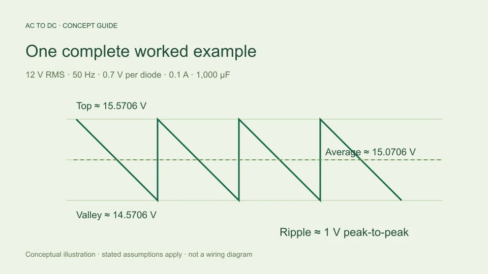
Choose a constant load current of 0.1 A, an input frequency of 50 Hz, and a capacitance of 1,000 µF. The approximate bridge discharge interval is 1/(2 × 50) = 0.01 s. Charge removed over that interval is 0.1 × 0.01 = 0.001 C.
Dividing by 0.001 F gives a voltage decline of 1 V. Using the combined formula produces the same result: 0.1 ÷ (2 × 50 × 0.001) = 1 V peak-to-peak. Calculating it both ways helps reveal which physical assumptions sit behind the compact expression.
At 60 Hz, with the same modeled current and capacitance, the approximate interval is 1/120 s. Ripple becomes about 0.8333 V p-p. The available top voltage is unchanged if the sinusoidal RMS input and diode-drop assumptions stay unchanged; only the estimated time for discharge has changed in this particular comparison.
Connect ripple to peak, valley, and average
For the filtered bridge, the calculator estimates available top voltage as Vtop ≈ √2 Vrms − 2Vf, clamped to zero if that expression is negative. Vf is the assumed drop of one conducting diode; the bridge path includes two.
With 12 V RMS and 0.7 V per diode, Vtop is about 15.5706 V. A 1 V discharge gives an estimated valley of 14.5706 V. If the decline is approximated by a straight line, its midpoint is about 15.0706 V, which is the estimated average for that simplified waveform.
Peak-to-peak ripple is the distance between top and valley, not the difference between top and average. In this example the top-to-average difference is 0.5 V, while the top-to-valley ripple is 1 V. Confusing these descriptions produces a factor-of-two error even when the underlying charge calculation was correct.
Compare changes one input at a time
The ripple equation allows clean sensitivity comparisons within its assumptions. Doubling current from 0.1 A to 0.2 A doubles estimated ripple from 1 V to 2 V. Doubling capacitance from 1,000 µF to 2,000 µF halves it from 1 V to 0.5 V. Doubling input frequency also halves the estimated discharge interval.
These comparisons describe a mathematical model with the other inputs held constant. In a physical circuit, a larger capacitor can change charging-current behavior and source loading. A changed load can affect transformer voltage and diode drop. Those effects are not silently included just because the arithmetic returns a result.
For useful comparisons, make a small table with one changed variable per row and record the resulting top, average, valley, and ripple. This distinguishes the equation’s direct sensitivity from assumptions about how the actual source and load behave. Avoid changing three settings together and then attributing the result to only one of them.
Know what the 20% guardrail means
The calculator rejects filtered cases when estimated ripple exceeds 20% of the available top. The threshold defines the tool’s chosen small-ripple scope. It does not claim that all accepted results are accurate within a particular percentage, nor does it establish a universal boundary between good and bad circuit designs.
For the 15.5706 V available top in the example, a 1 V ripple is approximately 6.42% of the top. That satisfies the model’s guardrail. A much smaller capacitor could make predicted ripple exceed the threshold. The tool then asks for changed conditions or a fuller simulation rather than presenting a simple midpoint estimate as though its assumptions still held.
The distinction matters because a calculated valley below zero would indicate that the assumed discharge model had broken down, not that an ordinary capacitor supply follows an unrestricted negative sawtooth. Rejecting an out-of-scope result protects the meaning of the estimate without pretending to solve the more complicated waveform.
Recognize the omitted circuit effects
The model assumes constant current during discharge. A resistor instead draws current proportional to its voltage, which produces an exponential discharge when isolated from the source. A downstream electronic load may have its own time-dependent behavior. Constant-current arithmetic should therefore be identified as an assumption rather than treated as a description of every possible load.
The model also omits capacitor equivalent series resistance, leakage, tolerance, and the source’s resistance. Diode characteristics and finite charging intervals affect how the capacitor is replenished. Transformer regulation can change the available input voltage with load. These are reasons to use device data and a more detailed circuit model when the simple estimate is insufficient.
An accepted voltage estimate does not select capacitor ripple-current capability, voltage rating, temperature suitability, or service life. Those are separate component questions. Likewise, reducing the predicted voltage ripple does not independently establish that all charging currents or thermal stresses are acceptable. The equation answers a deliberately narrower question about approximate discharge voltage.
Report a reproducible ripple estimate
A clear result states the input as sinusoidal RMS at the bridge terminals, identifies the frequency as AC input frequency, and lists load current, capacitance, and assumed diode drop. Report ripple as peak-to-peak voltage and distinguish the estimated average from the estimated valley.
For the example, a useful sentence is: “With a 12 V RMS, 50 Hz sinusoidal input, a filtered bridge using an assumed 0.7 V per diode, 0.1 A constant load, and 1,000 µF, the simplified model estimates 1 V p-p ripple and about 15.0706 V average.” That sentence carries enough context for another reader to reproduce the result.
If a measurement differs, first compare the model inputs and definitions rather than adjusting an unexplained multiplier. Check whether the current is approximately constant, whether RMS and peak were distinguished, and whether the capacitance units were converted. A transparent discrepancy is more useful than an apparently precise number detached from its circuit assumptions.
When comparing two estimates, retain their original assumptions in the record. A result using a fixed current and a result using an equivalent resistance may share the same nominal load point while describing different behavior during discharge. Matching one average number does not make the models identical. The waveform definition, timing interval, and input conditions explain what each result can legitimately support.
The same charge equation can also be rearranged for a mathematical capacitance estimate: C ≈ I/(2fΔVpp). For 0.1 A, 50 Hz, and a target of 0.5 V p-p, it gives 0.002 F, or 2,000 µF. This is a rearrangement under the same assumptions, not a component recommendation. A practical capacitor still has tolerance, voltage and current limits, thermal behavior, and other characteristics that the ripple expression does not choose.
Filed under rectifier basics worked examples