 AC/DC Calc
calculator guides
The limits of a simple AC to DC calculator
Learn which questions a rectifier estimate can answer, what its assumptions omit, and when the calculation needs a fuller model.
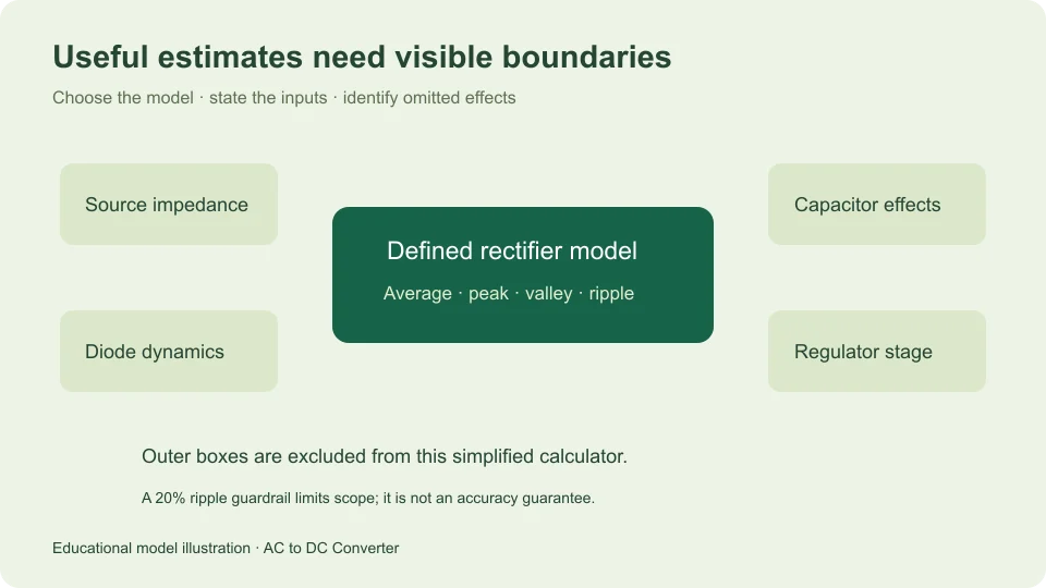
A simple AC-to-DC calculator is useful when its model matches the question being asked. It can convert a sinusoidal RMS input into an ideal rectifier average or estimate the discharge ripple of a defined capacitor-filtered bridge. It cannot reconstruct an unspecified power supply from one voltage number.
The most important limitation is therefore not the number of decimal places on screen. It is the gap between the circuit described by the inputs and the circuit whose behavior you want to understand. Reading the assumptions is part of using the result, rather than an optional note to visit after the answer looks surprising.
This guide describes the scope of the three models offered on this site. It separates exact relationships within ideal mathematical models from a deliberately simplified filter approximation, then explains what additional questions those models leave unanswered.
Define the quantity before choosing a formula
“DC output” can mean a waveform average, a capacitor’s highest recurring level, the lowest level between charging peaks, or a regulated output specification. These quantities need not agree. A single multiplier cannot answer all of them.
For a 12 V RMS sine, ideal full-wave average is approximately 10.8038 V, while its peak is approximately 16.9706 V. Add the site’s illustrative fixed-drop bridge and small-ripple capacitor model, and the estimated average can be around 15.0706 V under its default load and filter settings.
The different values come from different questions and assumptions. Comparing them without labels can make a correct formula appear wrong or a mismatched model appear accurate by coincidence. State whether the desired result is average, peak, valley, or ripple before deciding which mode is relevant.
Understand what is exact in an ideal model
For a sinusoidal input with peak Vm, an ideal full-wave output is Vm|sin θ|. Integrating over a complete cycle gives its average as 2Vm/π. An ideal half-wave output has average Vm/π when the blocked half-cycle remains in the averaging interval.
These are exact analytical results for the defined ideal waveforms. The relation Vm = √2 Vrms is likewise exact for a zero-offset sine. Numerical implementation and display introduce finite arithmetic and rounding, but those are distinct from changing the physical model.
Ideal here means zero forward diode loss, no smoothing capacitor, and the stated resistive-load waveform behavior. A real circuit does not become ideal because the analytical equation is exact. Calling the formula exact should always be accompanied by the conditions that make the mathematical waveform the one being analyzed.
Recognize the filtered model as an approximation
The capacitor-filtered bridge model starts with an available top of approximately √2 Vrms minus two fixed forward diode drops. It assumes that the capacitor is restored near each rectified crest, then discharges under approximately constant load current until the next charging opportunity.
Charge balance gives ΔV ≈ IΔt/C. Taking Δt as approximately 1/(2f) gives ΔVpp ≈ I/(2fC). Treating the discharge as linear gives average approximately top minus half the ripple, and valley approximately top minus all the ripple.
The capacitor charge relation and doubled bridge frequency appear in Texas Instruments TIDUB95, section 3.1. The midpoint average used here follows from the site’s assumed linear discharge picture. It is not a manufacturer guarantee of a particular physical output.
Interpret the 20% ripple guardrail correctly
The filtered calculator rejects a case when its estimated peak-to-peak ripple exceeds 20% of the available top. This is a product guardrail chosen to keep the small-ripple approximation within a limited operating scope. It is not a universal circuit design rule.
Nor does acceptance imply a certified percentage error. A case with 10% estimated ripple can still differ from hardware because source impedance, diode behavior, capacitor properties, or the load violates the assumptions. A threshold on one calculated ratio cannot bound every omitted effect.
If a case is rejected, increasing capacitance or reducing assumed current may bring the arithmetic into scope, but it does not by itself validate a hardware change. The alternative is to use a fuller circuit model that describes the behavior being studied. Do not suppress the rejection merely to obtain an attractive output number.
Source behavior is outside the fixed-input picture
The calculator accepts an RMS input value as given. It does not predict how that voltage changes as a transformer or another source supplies a changing load. Winding resistance, source impedance, regulation, and waveform distortion can affect the rectifier’s actual input and charging conditions.
For a sensitivity exercise, you can enter different justified RMS assumptions and see how the model’s output changes. That is useful for understanding the consequence of an input range. It does not calculate the range itself, and it does not reveal a source’s current capacity from voltage alone.
Hammond Manufacturing’s rectifier guide distinguishes rectifier and filter arrangements and explicitly notes losses beyond its ideal guide factors. Use source and component documentation for those omitted conditions rather than treating a simplified voltage equation as their replacement.
A fixed diode drop is a chosen input
The bridge mode subtracts two copies of a user-entered forward drop. The default 0.7 V per diode is illustrative. It is not a universal constant for every diode or operating condition, and it is not automatically extracted from a device datasheet.
Within this fixed-drop model, changing the input from 0.7 V to 0.5 V per diode raises the calculated top by 0.4 V. That arithmetic demonstrates sensitivity to the assumption. It does not predict the operating voltage of a named part, because the model does not solve the current and temperature dependence of its characteristics.
The ideal unfiltered modes deliberately omit diode drop entirely. They should not silently share a filtered-mode setting that their formulas do not use. Explicitly different models are clearer than one interface that applies an unexplained correction across unrelated formulas.
Real capacitors contribute more than capacitance
The filtered model treats the entered capacitance as a single fixed value. It does not model tolerance, leakage, ESR, temperature dependence, aging, or recharge-current heating. Those properties can matter even when the nominal capacitance is entered without a unit error.
The estimate also does not choose a capacitor voltage rating or permissible ripple current. The top and valley are waveform estimates under the assumed model, not complete component requirements. A practical rating decision needs the relevant operating extremes, component specifications, and application criteria.
Converting microfarads to farads correctly remains essential: 1,000 µF equals 0.001 F. But correct units solve only the scale problem. They do not turn an ideal capacitor parameter into a full physical component model.
Load behavior can change the discharge shape
The simplified filter mode uses constant current during discharge. A constant resistor instead draws current proportional to its instantaneous voltage. Other loads can switch, regulate, pulse, or change operating state. Their capacitor discharge behavior need not be the same linear ramp.
A hypothetical 0.1 A constant load is therefore a model statement. It is not proof that a connected device draws that current at every point in the ripple cycle. If the actual load changes substantially, a single assumed current may conceal the part of the waveform that matters most.
Startup and transient behavior are also excluded. The repeating steady-state approximation does not describe the complete charging process from an initially uncharged capacitor or a sudden change in load. A steady average is not a prediction of maximum transient stress or startup timing.
Regulated and switching supplies need their own models
A regulated adapter does more than rectify a sine and store charge. Its control and conversion stages determine output behavior within their specified conditions. The bridge calculation has no inputs describing those stages, so it cannot infer their output voltage or available current.
Likewise, three-phase rectification, controlled rectifiers, voltage multipliers, and half-wave capacitor filters require different waveform and circuit assumptions. A similar name is not enough reason to reuse the same equation. A useful calculator should identify exactly which topology it implements.
When the required circuit is outside the available modes, choose a model that accepts the necessary information instead of stretching the input labels. Renaming a peak measurement as RMS or treating a regulated output label as a rectifier input will produce numbers, but not an answer to the original question.
Treat a zero-load result as a limiting case
Entering zero current in the simplified filtered model produces zero calculated discharge ripple. That is the mathematical consequence of assuming no charge removal by the load. It does not assert that an actual capacitor and circuit have no leakage or other current paths.
The tool also treats zero available bridge top and zero assumed load as a zero-output limiting case, while rejecting a positive assumed load when the modeled input peak cannot overcome the diode drops. These rules make the arithmetic behavior explicit at the boundary; they do not model the complete low-voltage behavior of real diodes.
Use results as reproducible, qualified statements
A strong result includes its inputs, selected mode, units, and meaning. For example: “Approximately 15.0706 V average under the filtered bridge model, using 12 V RMS sinusoidal input, 50 Hz, 0.7 V per diode, 0.1 A constant load, and 1,000 µF.” That statement can be reproduced and questioned intelligently.
Keep numerical verification separate from physical validation. Unit tests and worked examples can show that software implements its stated equations. They cannot establish that an unspecified physical circuit satisfies the assumptions. Conversely, an observed mismatch does not identify an arithmetic bug until the conventions and circuit scope have been compared.
Use the main calculator for its defined questions, the worked formulas guide for derivations, and the measurement guide for interpreting reported quantities. The most useful output is a well-described estimate whose limits remain visible alongside the number.
Filed under calculator guides