AC/DC Calc
measurement guides
Measuring rectifier output: know which voltage you mean
Interpret DC average, ripple, peak, and RMS readings without confusing one measurement with another.
A rectifier output can have several legitimate voltage values at the same time. Its average might be 15 V, its top might be higher, and its valley might be lower. An instrument reporting the varying part of that signal may show a much smaller number. None of those values can be interpreted correctly without knowing the measurement convention.
The useful starting question is therefore more specific than “What is the DC voltage?” Ask whether you need the average level, the lowest point between charging peaks, the total RMS value, or the ripple amplitude. This guide explains those distinctions and a way to organize the information around a reading. It is not a procedure for connecting instruments to live equipment or a substitute for an instrument’s instructions.
Start with a description of the output
An ideal unfiltered full-wave rectifier produces a positive sequence of sine-shaped humps. The waveform falls to zero between humps. Calling it DC describes its one-direction polarity, but does not make it a flat voltage. Its complete-cycle average is lower than its peak, and its RMS value differs from that average.
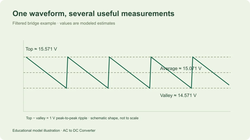
A bridge followed by a smoothing capacitor produces a different shape. In a simplified picture the capacitor charges near a crest, then supplies the load while the rectified source falls below it. The voltage decreases until the next recharge. This waveform can have a large positive average with a smaller variation around that level.
A regulated supply adds another stage and can behave differently again. Before comparing an observed result with a calculator, write down which of these arrangements is being described. A correct calculation for an unfiltered waveform is the wrong reference for a filtered supply, even when both start with the same AC input.
Separate average, top, valley, and ripple
Average voltage is the signed area under the waveform divided by the observation time. For a repeating signal, one complete period is enough mathematically, although a practical measurement may use many periods. In the filtered model on this site, the discharge is approximated as linear, so its midpoint is used as an estimate of the average.
The top is the highest recurring voltage in that model. The valley is the lowest recurring voltage before recharge. Peak-to-peak ripple is the difference between them: top minus valley. It is an amplitude description, not an RMS reading and not the frequency at which the pattern repeats.
For example, a top of 15.6 V and valley of 14.6 V imply 1.0 V peak-to-peak ripple. A linear ramp between those levels has a midpoint of 15.1 V. The 1.0 V variation and the 15.1 V average describe the same waveform from different perspectives. Replacing one with the other loses essential information.
Know what an instrument function includes
The words AC, DC, and RMS on an instrument need to be read with its documentation. An AC measurement may exclude the DC component, whereas another function may include both components in a total RMS result. “True RMS” by itself does not identify which components are included in every operating mode.
Fluke’s discussion of true-RMS measurement distinguishes AC-coupled readings from combined AC-plus-DC RMS capability. That distinction is relevant when interpreting ripple riding on a positive DC level.
Keep the exact function name in your notes. A record saying only “AC range” or “DC volts” may be insufficient for a later comparison. Instrument bandwidth, allowed waveform characteristics, specified range, and accuracy conditions also belong to the measurement context; their values are specific to the instrument, rather than universal properties of rectifiers.
Use a calculation as a defined reference
Consider a hypothetical single-phase sinusoidal input of 12 V RMS feeding a bridge and capacitor. Choose 0.7 V as the illustrative forward drop of each conducting diode, 50 Hz input frequency, 0.1 A constant load, and 1,000 µF capacitance. These are stated model inputs, not measured characteristics of a particular power supply.
The sine peak is 12 × √2, approximately 16.9706 V. Subtracting two assumed diode drops gives an available top of approximately 15.5706 V. Converting 1,000 µF to 0.001 F, the small-ripple estimate is 0.1/(2 × 50 × 0.001), or 1 V peak-to-peak.
The resulting estimated valley is 14.5706 V, and the estimated midpoint average is 15.0706 V. If the quantity of interest is the valley, compare against the valley estimate. If it is the average, use the average estimate. A comparison against the 16.9706 V input crest would answer a different question.
Record the input at the correct location
The calculator needs the AC RMS voltage at the rectifier input. In a transformer-fed example, that means the voltage associated with the winding feeding the rectifier, not a number describing a different winding or a nominal system label. A ratio between windings is separate information and is not inferred by the calculator.
The description must also say that the input is sinusoidal. The relation peak = √2 × RMS follows from a sine wave; it is not a general conversion for every waveform. A signal with flattened peaks, pulses, or substantial distortion may have a different ratio.
Frequency is another independent input. It sets the time between recharge opportunities in the simplified filtered model. A 50 Hz sinusoidal input gives a full-wave repetition frequency of 100 Hz; 60 Hz gives 120 Hz. Mixing the input frequency with the already doubled ripple frequency in the formula creates an avoidable factor-of-two error.
Compare like operating conditions
A rectifier output is connected to a load, and that load affects a capacitor-filtered waveform. The default model treats the load as a constant current. A reading taken under another condition cannot be treated as a direct check of that model without describing the difference.
For example, changing the assumed current from 0.1 A to 0.2 A doubles the calculated discharge ripple when frequency and capacitance stay fixed. The modeled top remains unchanged, but the valley and average decrease. This is a consequence of the simplified assumptions, not a claim that every real supply will keep exactly the same top under extra load.
Write whether the values describe a steady condition or a changing one. Startup, intermittent loads, and transitions may not resemble the repeating steady waveform used in the calculation. A single displayed voltage can hide those distinctions. Recording the observation interval makes the intended comparison clearer.
Distinguish disagreement from a failed model
A difference between a calculated and observed result can arise for several reasons. The chosen quantity might be wrong, the input convention might be mismatched, or the real circuit might include effects that the simplified model excludes. Arithmetic is only one possible source of disagreement.
Start by checking labels and units on paper. Was the input RMS rather than peak? Was the capacitance expressed in microfarads before conversion to farads? Was the current in amperes rather than milliamperes? Were both conducting bridge diode drops included? These checks examine the description and calculation without requiring a new hardware action.
Next compare scope. The model excludes source impedance, transformer regulation, changing diode drop, capacitor ESR, and regulator behavior. A circuit containing significant contributions from those effects deserves a more complete analysis. Adjusting an unrelated input until the displayed answer matches a reading can conceal the actual reason for the difference.
Preserve precision without overstating confidence
The calculator may display several decimal places so that differences between examples remain visible. Those digits do not demonstrate that a physical output is known to that resolution. A model with an illustrative 0.7 V diode assumption cannot acquire laboratory precision merely because its arithmetic uses more digits.
Retain enough digits during intermediate calculations to avoid unnecessary rounding error, then report an appropriately qualified final result. “Approximately 15.1 V average under the stated model” communicates more than an unexplained string of decimals. Keep the input values and assumptions with the result so someone else can reproduce it.
Do not interpret the peak or valley estimates as component ratings or electrical safety assessments. Those decisions depend on information the model does not accept. The purpose of recording the measurements clearly is to understand the quantity, not to expand the calculator into an equipment qualification tool.
Keep arithmetic checks separate from observations
It is useful to maintain two clearly labeled columns when reviewing a result: values observed with an identified instrument function, and values inferred from a mathematical model. A voltage that was calculated from another reading is not an additional independent measurement. Keeping that distinction visible prevents several derived numbers from looking like multiple pieces of confirming evidence.
For the default example, top, valley, and midpoint are linked by one assumed ripple span. Agreement among those three calculated numbers checks internal consistency. It does not provide three separate validations of the actual output waveform.
Build a reproducible comparison note
A useful note has four parts: circuit description, calculator inputs, reported quantities, and observation conditions. For this example it would identify a sinusoidal single-phase bridge with smoothing capacitor, list all five numeric inputs, and distinguish average, top, valley, and peak-to-peak ripple.
If an instrument reading is included, add the function name and the relevant measurement convention. Describe any known differences between the circuit and the calculator assumptions. Keep independently measured values separate from values inferred by calculation; combining them in one unlabeled list makes later review harder.
Use the AC to DC calculator to reproduce the example and the RMS, peak, and average guide for the definitions behind it. For another comparison, the ideal full-wave tool deliberately omits the capacitor and diode losses. Its different answer illustrates why the model description belongs beside every useful voltage result.
Filed under measurement guides