AC/DC Calc
measurement guides
Rectifier average versus RMS output: calculate both correctly
Derive why a rectified waveform can have one average, another RMS value, and a separate ripple component.
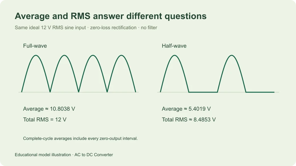
An ideal full-wave rectifier supplied by a 12 V RMS sine has approximately 10.8038 V average output and 12 V total RMS output. Those values describe the same positive waveform. The difference is not a contradiction or an unexplained loss; average and RMS are different mathematical operations.
The average describes the signed area per unit time. RMS describes the square root of the mean squared voltage. Rectification changes the sign pattern, and that affects these operations differently. Working through the definitions is more reliable than treating every quantity labeled “DC” as interchangeable.
This article considers ideal zero-drop rectifiers with no smoothing capacitor and a resistive load. A capacitor-filtered output is introduced separately to show why its waveform cannot inherit the unfiltered formulas automatically. The examples are analytical calculations, not reports of measured hardware performance.
Define the waveform before the statistic
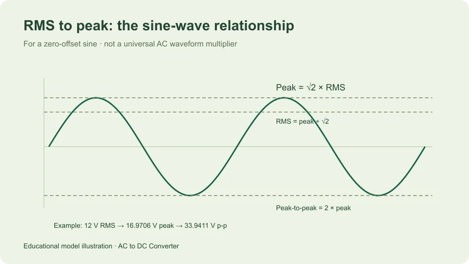
Write the input as v(θ) = Vm sin θ over a complete cycle from 0 to 2π. Its peak magnitude is Vm, and its RMS is Vm/√2. The signed average of that input sine is zero because the positive and negative areas cancel.
An ideal full-wave output is y(θ) = Vm|sin θ|. It retains every input magnitude and makes the negative half-cycle positive. Its period is half the input period, although averaging over a complete input cycle gives the same answer as averaging over one output period.
An ideal half-wave output is Vm sin θ during the positive half-cycle and zero during the negative half-cycle. It therefore contains a full interval with no output. Keeping that zero interval in the averaging window is essential; leaving it out would calculate a conditional average over conduction rather than the complete-cycle average.
Derive the full-wave average
The area under sin θ between zero and π is 2. Full-wave rectification provides two such positive areas in a complete input cycle, so the total normalized area is 4. Multiplying by Vm and dividing by the cycle length 2π gives Vavg = 2Vm/π.
Substitute Vm = √2 Vrms,input to obtain Vavg = (2√2/π) Vrms,input. The coefficient is approximately 0.900316. For a 12 V RMS input, the average is approximately 10.8038 V.
This is an average of a pulsating voltage. The ideal waveform still reaches zero between peaks, and its peak is approximately 16.9706 V in the example. The average does not describe its minimum or establish that a load sees a nearly constant supply.
Derive the full-wave RMS
Squaring removes the effect of sign: |sin θ|² equals sin² θ. The ideal full-wave output therefore has exactly the same squared waveform as its sine input. Its mean square remains Vm²/2, and its total RMS is Vm/√2.
For the 12 V RMS input example, full-wave output RMS is consequently 12 V. The ideal rectifier changes polarity without discarding either half-cycle’s magnitude. There is no need to invoke an empirical multiplier to obtain this result; it follows immediately from the definition.
The ratio of total RMS to average is π/(2√2), approximately 1.11072. That ratio belongs to this specific unfiltered full-wave shape. It should not be carried into a filtered bridge waveform or another rectifier configuration merely because each output is unidirectional.
Derive the half-wave values
For half-wave rectification, only the positive sine area contributes. Its area is 2Vm over a complete input cycle of length 2π, giving Vavg = Vm/π. With a 12 V RMS sine input, that is approximately 5.4019 V.
For RMS, integrate the squared sine over only the conducting half-cycle, while retaining the full cycle in the denominator. The integral of sin² θ from zero to π is π/2. The resulting mean square is Vm²/4, so output RMS is Vm/2.
Since input RMS is Vm/√2, ideal half-wave output RMS is input RMS divided by √2. The example gives approximately 8.4853 V RMS. Its average is half the full-wave average, but its RMS is not half the full-wave RMS because the square-root operation changes the scaling relationship.
Keep the numerical comparison together
For the same 12 V RMS sinusoidal input, all three waveforms have a peak magnitude of approximately 16.9706 V. The original sine averages to zero and has 12 V RMS. The full-wave output averages to approximately 10.8038 V and retains 12 V RMS. The half-wave output averages to approximately 5.4019 V and has approximately 8.4853 V RMS.
This comparison separates the waveform from the summary statistic. If a question asks for complete-cycle average DC output, use the average column of that mental comparison. If it asks for total RMS output under the stated ideal model, use the RMS relationship instead.
Do not compare one result’s average with another result’s RMS and call the difference an efficiency. Electrical efficiency concerns power supplied and delivered with appropriate current and circuit information. A ratio of two differently defined voltage statistics does not by itself provide that answer.
Separate DC average from the remaining ripple
Any periodic waveform can be written as its average D plus a zero-mean remainder r(t). Expanding the square gives (D + r)² = D² + 2Dr + r². The mean of the cross term is zero because r has zero mean.
Therefore total RMS squared equals D² plus the RMS of the zero-mean remainder squared. Rearranging, ripple RMS = √(total RMS² − average²), provided both terms describe the same waveform and observation interval.
For the ideal full-wave example, ripple RMS is √(12² − 10.8038²), approximately 5.2228 V using unrounded intermediate values. This is not its peak-to-peak ripple, which spans zero to the 16.9706 V peak. RMS amplitude and peak-to-peak amplitude remain distinct even after the DC component has been separated.
Why instrument modes matter here
A measurement labeled AC RMS may report the varying component after removal of the DC level. A combined AC-plus-DC RMS function may report the total instead. Those are different quantities for the same rectifier output, so their readings need not match.
Keysight’s true-RMS measurement guidance notes that AC coupling rejects a DC component. Match the instrument function to the quantity being compared rather than relying on the word RMS alone.
The Fluke 287/289 manual describes separate AC and DC component readings and a combined AC-plus-DC RMS option for those instruments. That is a device-specific example, not a claim that every meter provides the same functions or performance.
A filtered output needs a new waveform model
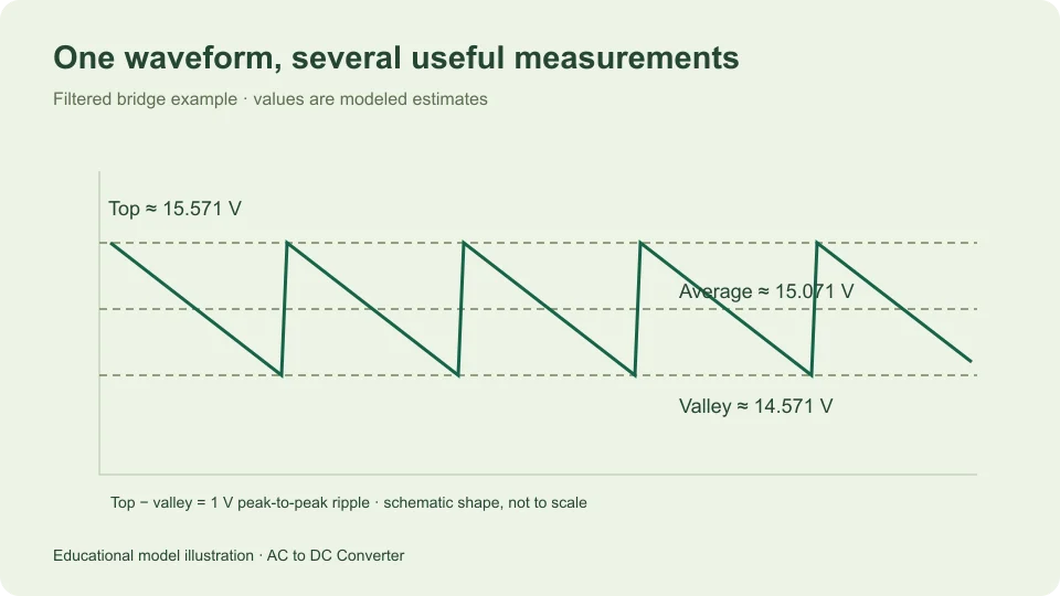
A smoothing capacitor changes the output shape rather than simply relabeling the unfiltered sine. Under the site’s simplified constant-current model, it discharges approximately linearly between rapid recharges. Its average is estimated from the midpoint between top and valley.
Suppose that model gives a top of 15.5706 V and valley of 14.5706 V. The estimated average is 15.0706 V, with 1 V peak-to-peak ripple. For an ideal linear sawtooth centered on its mean, the varying component has RMS equal to its peak-to-peak span divided by √12, approximately 0.288675 V in this example.
That additional RMS relationship belongs to an assumed linear ramp, not the exact waveform of every capacitor-filtered bridge. The main calculator does not display it as a measured or guaranteed result. Finite charging intervals, source resistance, and changing load can alter the shape.
Use constant voltage as a limiting comparison
A perfectly constant voltage D has average D and RMS magnitude |D|. For a positive constant supply, the two numerical values agree because every point on the waveform has the same value. Its zero-mean ripple component is zero. This is the special case that can make it tempting to assume average and RMS always mean the same thing in DC discussions.
Now add a small zero-mean variation while preserving the same average. Its mean squared contribution is positive, so total RMS increases above the average magnitude. The difference can be small when ripple is small, but the mathematical distinction remains. For a 15 V average and 0.3 V ripple RMS, total RMS is √(225 + 0.09), approximately 15.0030 V. That near agreement does not mean the ripple vanished.
This limiting comparison explains why the distinction may be easy to miss in a well-smoothed numerical example and very visible in an unfiltered rectifier. Describe the quantity explicitly in both cases. A rounded display can make two values look identical even though their underlying definitions and their usefulness for another calculation remain different.
Preserve the observation interval
The mathematical results above average complete repeating cycles. Selecting only part of a waveform can change both average and RMS because the included values have changed. A window centered around a crest is not equivalent to one containing an entire cycle, even though both observations concern the same periodic signal.
When comparing a theoretical result with recorded data, keep the averaging interval and any gating or component removal explicit. This article’s numerical values refer to complete-cycle ideal waveforms. They should not be used as reference values for an unspecified partial-cycle statistic without first reconciling the definitions.
Avoid common averaging mistakes
One common mistake is averaging only the nonzero half-wave interval and forgetting the blocked interval. Another is assuming that a full-wave rectifier’s total RMS falls by the same factor as its average. A third is calling the RMS of the varying component the total output RMS without saying that the DC level was removed.
Write the waveform definition and averaging interval first. Then state whether you are finding an average, total RMS, or RMS after removal of the mean. Keep volts, waveform convention, and circuit model beside the result.
The ideal full-wave calculator and ideal half-wave calculator report the appropriate average, peak, valley, and repetition rate for their defined models. The main AC to DC tool adds the filtered approximation. Its explanations help keep a useful average estimate separate from a claim about smoothness, regulation, or available power.
Filed under measurement guides