Half-Wave vs Full-Wave Rectifiers: Compare the Same Quantities

Half-wave and full-wave rectifiers can be compared meaningfully only when the same input, output quantity, and assumptions are used. A peak from one circuit should not be compared with an average from another as though both numbers described the same property. Filtering also changes the output waveform and must be identified separately.

This guide begins with ideal zero-drop diodes, no smoothing capacitor, a resistive load, and sinusoidal single-phase input. These are the assumptions behind the site’s half-wave calculator and full-wave calculator. The comparison then explains how a filter changes the questions a calculator needs to answer.

Start with one common input

Write the input voltage as v = Vm sin θ. Vm is its positive peak. For a sine, input RMS is Vm/√2, so Vm = √2 Vrms. This establishes the same source waveform for both ideal rectifier calculations.

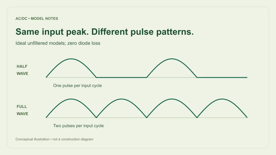
A half-wave rectifier passes one polarity and blocks the other. Its ideal output is the positive half-sine followed by a zero-output interval. A full-wave rectifier directs both input half-cycles to the same output polarity. Its ideal output is the absolute value of the original sine.

Neither operation increases the surviving ideal crest. Both outputs reach Vm when their conducting half-sine reaches its peak. Their difference lies in which parts of the input cycle contribute output and how often those positive pulses occur. That difference affects averages and timing even though the peak amplitude is the same.

Complete-cycle average explains the factor of two

For half-wave output, the positive half-sine has area 2Vm over the angle interval 0 to π. The remaining half-cycle contributes zero. Dividing by the full 2π input cycle gives Vavg,half = Vm/π.

For full-wave output, there are two identical positive half-sine areas in the same input cycle. Their combined area is 4Vm. Dividing by 2π gives Vavg,full = 2Vm/π. The ideal full-wave complete-cycle average is therefore exactly twice the ideal half-wave average for the same input peak.

The interval is essential. Averaging the conducting half of the half-wave signal alone would give 2Vm/π, but that excludes the blocked interval and is not the complete-cycle mean used here. If two sources report different “averages,” check whether they average over the same interval before deciding that one formula is incorrect.

Express the averages in terms of RMS input

Substitute Vm = √2 Vrms. Ideal half-wave average becomes √2 Vrms/π, approximately 0.450158 Vrms. Ideal full-wave average becomes 2√2 Vrms/π, approximately 0.900316 Vrms.

For a 12 V RMS input, the ideal half-wave average is approximately 5.4019 V. The ideal full-wave average is approximately 10.8038 V. Both have an ideal peak of approximately 16.9706 V and a valley of zero. These numbers describe pulsating output, not a smooth regulated DC supply.

The rounded resistive-load factors of about 0.45 and 0.90 appear in Hammond Manufacturing’s rectifier design guide. The guide also distinguishes filter arrangements, reinforcing why an ideal unfiltered comparison should not be silently extended to capacitor-input results or other rectifier topologies.

Output RMS is a separate comparison

RMS depends on the average of squared voltage. Full-wave rectification changes signs but not squared values, so ideal full-wave output RMS equals the original sine RMS. A 12 V RMS sine therefore remains 12 V RMS after ideal full-wave rectification.

For half-wave output, only one half-cycle contributes squared voltage over the complete input cycle. The mean square is Vm²/4, giving output RMS Vm/2. With the same 12 V RMS sine input, that is approximately 8.4853 V RMS.

The ratio of output RMS values is therefore √2, while the ratio of complete-cycle averages is two. There is no contradiction because RMS and average perform different mathematical operations. This is a useful example of why a single unqualified “output voltage” number can be misleading. State which quantity is being compared and retain the waveform assumptions with it.

Ripple repetition differs from ripple amplitude

In ideal half-wave rectification, there is one positive pulse per AC input cycle. The output pattern repeats at f, the original AC frequency. With full-wave rectification, there are two positive pulses per input cycle, so the pattern repeats at 2f.

At 50 Hz AC input, ideal half-wave pulses repeat every 20 ms and full-wave pulses every 10 ms. At 60 Hz, the corresponding intervals are approximately 16.667 ms and 8.333 ms. These intervals describe when pulses occur rather than how large their voltage variation is.

For both unfiltered ideal models, the valley is zero and the peak is Vm. Their peak-to-peak waveform variation is therefore Vm. Full-wave output has a higher repetition frequency and a higher average, but its ideal zero-to-peak amplitude span is not halved. Frequency, average, and peak-to-peak ripple are distinct comparison quantities.

A filter changes the waveform being compared

A capacitor can support the output between charging crests by supplying stored charge to the load. Under a simple constant-current assumption, voltage decline follows ΔV ≈ IΔt/C. The longer the interval between replenishing peaks, the larger the estimated decline when the other assumptions are held constant.

Using a full input cycle as an approximate half-wave discharge interval gives I/(fC). Using half an input cycle for full-wave gives I/(2fC). This timing comparison suggests half as much ripple for full-wave under otherwise matched simplified conditions, but it does not establish that two actual supplies share the same top voltage, diode losses, source loading, or charging behavior.

The site’s main calculator implements the capacitor-filtered bridge model, not a filtered half-wave model. Its ideal half-wave mode must not be interpreted as though the capacitor fields apply to it. Those fields are hidden and ignored in the ideal modes to keep the model boundary explicit.

Compare a numerical case carefully

Begin with 12 V RMS, 50 Hz, ideal zero-drop diodes, and no filter. Report half-wave as approximately 5.4019 V complete-cycle average, 16.9706 V peak, zero valley, and 50 Hz pulse repetition. Report full-wave as approximately 10.8038 V average, the same peak and valley, and 100 Hz repetition.

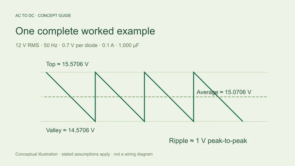
For a separate filtered bridge calculation, add assumptions of 0.7 V per diode, 0.1 A constant load, and 1,000 µF. Estimated top becomes 15.5706 V, ripple 1 V p-p, average 15.0706 V, and valley 14.5706 V. This is not simply the ideal full-wave result with a small correction; the capacitor changes the shape being averaged.

When making a comparison table, put these assumptions in a dedicated column. A filtered bridge average and an unfiltered half-wave average can both be useful, but their numerical ratio does not isolate the effect of rectification alone. More than one circuit feature has changed between those rows.

Do not infer component suitability from ideal averages

The ideal formulas provide waveform reference values. They do not determine available load current, transformer capability, diode reverse-voltage margin, charging-current stress, capacitor ratings, or thermal behavior. Voltage arithmetic is only one part of understanding a power circuit.

A physical bridge includes a pair of conducting diode drops, while another topology can have different conduction paths and source arrangements. Assuming a fixed diode drop can help a defined estimate, but it does not replace the device’s operating data. Source resistance and transformer regulation also affect the voltage available under load.

The filtered calculator further limits its approximation to cases whose estimated ripple is no more than 20% of its available top voltage. That is a tool-specific guardrail, not a universal performance boundary. A full simulation or measurement can be needed even for an accepted result when omitted physical effects materially affect the question.

Choose the calculator that matches the question

Use the ideal half-wave model when the question asks for the complete-cycle average of an ideal unfiltered half-wave sine. Use the ideal full-wave model for its full-wave counterpart. Use the filtered bridge estimate only when its sinusoidal input, constant-current load, fixed diode drop, and small-ripple assumptions fit the intended calculation.

Before comparing results, check five things: the same RMS input definition, the same measurement location, the same output quantity, the same filter condition, and the same loss assumptions. This often resolves an apparent disagreement more quickly than recalculating with additional decimal places.

The central comparison is simple but precise. Full-wave rectification uses both input half-cycles, which doubles the ideal complete-cycle average and doubles pulse repetition relative to half-wave at the same input. Peaks, RMS values, filtered behavior, and practical component requirements remain separate questions that deserve their own labels and models.

Build a comparison worksheet that preserves definitions

Use one row for each output quantity rather than one large “DC voltage” cell. Suggested rows are input RMS, input peak, complete-cycle output average, output RMS, output peak, output valley, and pulse repetition frequency. State “ideal, zero diode drop, no capacitor” at the top so the numerical comparison remains attached to its assumptions.

For a second input amplitude, scale the voltage rows proportionally while leaving frequency rows unchanged. If the 12 V RMS input becomes 6 V RMS, the ideal averages become about 2.7009 V half-wave and 5.4019 V full-wave. Their peaks both become about 8.4853 V. At the same input frequency, their repetition timing does not change.

For a second input frequency, do the opposite: keep the ideal voltage rows unchanged while updating pulse timing. This reveals which part of the comparison follows amplitude and which part follows time. It also provides an independent way to spot a spreadsheet reference error or an incorrectly entered frequency.

Only add a filtered row when its extra assumptions are available. Include per-diode drop, load current, capacitance, and model scope beside that row. This prevents a table from looking like an apples-to-apples rectification comparison when it also changes filtering and loss assumptions. The worksheet then becomes a transparent explanation rather than a collection of similar-looking but incompatible voltage numbers.

Filed under rectifier basics worked examples

Topics: half-wave · full-wave · waveform comparison