Rectifier Ripple Frequency: Why Full-Wave Output Repeats at 2f

Ripple frequency describes how often a repeating variation occurs. It does not describe how many volts the output changes by. Keeping those two ideas separate makes rectifier calculations much easier to interpret, particularly when a capacitor-ripple equation already includes a factor of two.

For the single-phase sinusoidal models on this site, ideal half-wave output repeats at the AC input frequency f, while ideal full-wave output repeats at 2f. A filtered bridge retains two charging opportunities per input cycle under the same basic model. This guide derives the timing, works through 50 Hz and 60 Hz examples, and explains where those simple relationships should not be extended.

Frequency and period describe the same timing differently

Frequency is the number of repetitions per second. Period is the time required for one repetition. They are reciprocals: T = 1/f and f = 1/T. Hertz means repetitions per second.

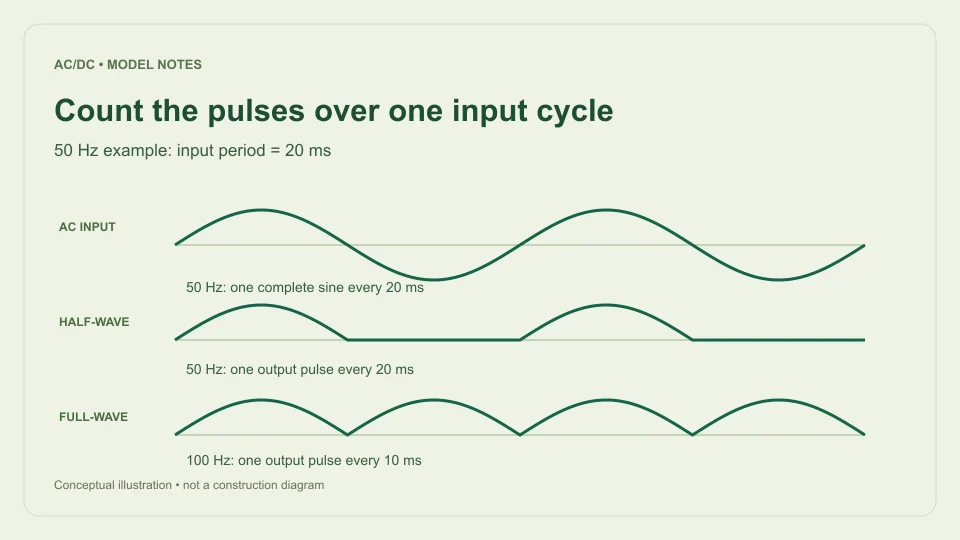
A 50 Hz input has a period of 1/50 s, or 20 ms. A 60 Hz input has a period of 1/60 s, approximately 16.667 ms. Each complete sine cycle contains a positive half-cycle and a negative half-cycle, so its crests of opposite polarity are separated by half the input period.

These time relationships do not depend on the sine’s amplitude. A 5 V RMS sine and a 12 V RMS sine at the same frequency have different voltage scales but the same timing. Changing the modeled RMS voltage alone therefore does not change the ripple frequency returned by an ideal rectifier model.

Half-wave output has one pulse per input cycle

An ideal half-wave rectifier passes one half of the sine and blocks the other. The resulting output has one positive half-sine followed by a zero interval. The next identical positive pulse occurs one complete input period later.

Its output pattern therefore repeats at f. For 50 Hz input, there is one pulse every 20 ms, giving a 50 Hz repetition frequency. For 60 Hz input, there is one pulse every approximately 16.667 ms, giving 60 Hz repetition.

The missing half-cycle is part of the output pattern. Ignoring that interval would incorrectly treat the half-sine itself as the full repeating period. It would also lead to the wrong averaging interval when calculating DC mean. The half-wave calculator uses the complete input cycle both for its average definition and for its pulse-repetition interpretation.

Full-wave output has two pulses per input cycle

Ideal full-wave rectification changes the negative half-cycle to positive output polarity. A positive output pulse now occurs for each input half-cycle. The sequence repeats after half the original input period because the reflected negative half has the same shape as the positive half.

Its output period is therefore T/2, and its repetition frequency is 1/(T/2) = 2/T = 2f. At 50 Hz AC input, the output pulses are 10 ms apart and repeat at 100 Hz. At 60 Hz input, they are approximately 8.333 ms apart and repeat at 120 Hz.

This is a timing consequence of using both half-cycles, not an extra oscillation introduced by a capacitor. The ideal full-wave waveform already has the doubled repetition frequency before smoothing is considered. The full-wave calculator reports that value alongside its ideal waveform average, peak, and valley.

A capacitor changes shape, not the number of input crests

A smoothing capacitor stores charge near a rectified crest and supplies the load between later charging intervals. Under the simplified bridge model, replenishment opportunities still occur twice per AC input cycle. The capacitor changes the output between those crests rather than creating an unrelated low-frequency timing source.

Texas Instruments TIDUB95, section 3.1, identifies the doubled frequency for a full bridge when deriving a smoothing-capacitor relationship from charge and discharge time. The site’s filtered bridge calculator uses that same timing assumption in its simplified ripple estimate.

Real charging takes a finite interval and depends on the source and load. The output waveform is not required to be a perfect sawtooth. The timing approximation is useful for a small-ripple estimate, but it does not by itself specify conduction angle, charging-current peaks, or every spectral component a measurement might show.

Put the correct frequency into the ripple equation

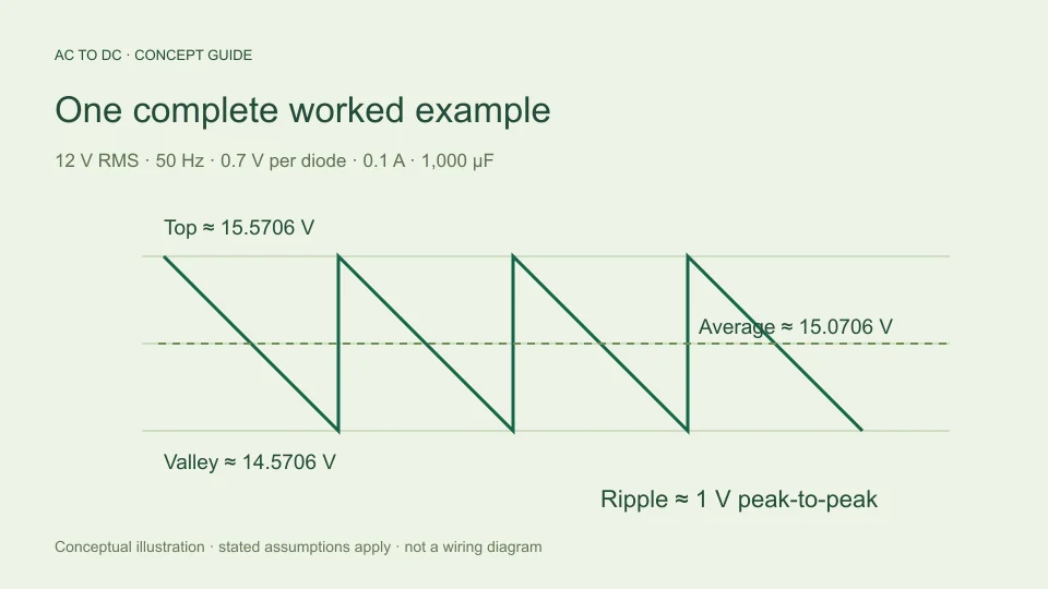
For a constant-current discharge approximation, ΔV ≈ IΔt/C. Using the approximate full-wave interval Δt ≈ 1/(2finput) gives ΔVpp ≈ I/(2finputC). If ripple frequency fripple is defined separately as 2finput, the equivalent expression is ΔVpp ≈ I/(frippleC).

These are the same equation written with different frequency definitions. Problems arise when a user enters the doubled ripple frequency into a field labeled AC input frequency and then retains the extra factor of two in the denominator. That counts the full-wave timing advantage twice and underestimates ripple by a factor of two.

For example, with 50 Hz input, 0.1 A, and 1,000 µF, use 0.1/(2 × 50 × 0.001) = 1 V p-p. Alternatively use 0.1/(100 × 0.001) = 1 V p-p with ripple frequency. Using 0.1/(2 × 100 × 0.001) would incorrectly produce 0.5 V for those assumptions.

Compare 50 Hz and 60 Hz under matched assumptions

Hold RMS voltage, load current, capacitance, and assumed diode drop constant. With a full-wave bridge at 50 Hz input, the simplified discharge interval is 10 ms. At 60 Hz, it is approximately 8.333 ms, which is five sixths as long.

Because the constant-current ripple estimate is proportional to discharge time, estimated ripple at 60 Hz is five sixths of the 50 Hz estimate. If the 50 Hz case gives 1 V p-p, the 60 Hz case gives approximately 0.8333 V p-p. This comparison follows directly from the model’s timing assumptions.

The modeled available top does not change merely because frequency changed if the sinusoidal RMS input and fixed diode-drop assumptions are unchanged. Estimated average and valley move because the modeled ripple changes. A physical source can have frequency-dependent behavior outside this simple comparison; the calculator does not silently include those additional effects.

Ripple frequency is not ripple percentage

Frequency answers how often the pattern repeats. Peak-to-peak ripple answers the voltage difference between its top and bottom. Ripple percentage is a ratio that requires a stated denominator, such as peak-to-peak ripple divided by average DC or by available top voltage.

At the same 100 Hz repetition frequency, two filtered bridge models can have very different ripple voltages because their load currents or capacitances differ. Conversely, changing voltage amplitude in an ideal unfiltered waveform changes its peak-to-peak variation without changing its repetition frequency.

This site’s 20% filtered-ripple guardrail compares estimated peak-to-peak ripple with available top voltage. That is a model-scope check, not a frequency setting and not a universal definition of ripple factor. Do not compare percentages from two tools unless they use the same numerator, denominator, waveform assumptions, and output quantity.

Repetition frequency and harmonics are different descriptions

A nonsinusoidal repeating waveform can be represented by a DC component plus sinusoidal components at integer multiples of its fundamental repetition frequency. The repeated full-wave shape is not a pure 100 Hz sine just because its fundamental pattern repeats at 100 Hz for 50 Hz input.

The ideal full-wave waveform contains a mean component and varying components consistent with its half-input-period repetition. A filtered waveform has a different shape and therefore a different distribution of those varying components. Source asymmetry or other real effects can also alter what appears in a measured spectrum.

The calculator reports the model’s basic ripple repetition frequency. It does not perform Fourier analysis, estimate harmonic amplitudes, predict electromagnetic interference, or identify every frequency a measurement may contain. If a measured component appears at a different frequency, investigate the actual waveform and measurement context rather than assuming that the calculator has described the entire spectrum.

Keep the model boundaries visible

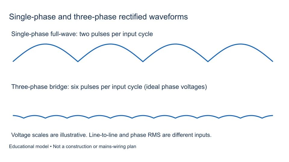
The f and 2f relationships here concern single-phase half-wave and full-wave rectification of the specified input. Three-phase rectifiers, switching converters, controlled conduction, and other topologies can require different timing models. A similar name does not justify reusing the same ripple equation.

The AC to DC formula guide shows how timing combines with the selected waveform or capacitor assumptions. Its filtered model also excludes source impedance, diode dynamics, capacitor ESR, and regulator behavior. The frequency relationship is one part of that model, not a complete power-supply prediction.

For a clear result, write “50 Hz AC input; 100 Hz bridge ripple repetition” rather than an unexplained “100 Hz.” Keep the input frequency label intact when entering a calculator, and use the equivalent ripple-frequency equation only when its definition is explicit. This small labeling discipline prevents a common factor-of-two error and makes the resulting estimate much easier to check.

Check timing with a simple pulse timeline

Mark an input cycle from 0 to 20 ms for a 50 Hz example. Positive input crests occur once in that interval, and negative crests occur halfway between successive positive ones. After ideal full-wave rectification, both become positive output crests. The interval between neighboring output crests is 10 ms, which corresponds to 100 Hz.

Now remove every alternate output pulse to represent the ideal half-wave pattern. The remaining neighboring crests are 20 ms apart, so repetition returns to 50 Hz. This timeline is a useful independent check because it does not rely on remembering whether a particular formula contained a two.

When examining a measured trace, identify what event repeats before converting its spacing into frequency. Two visible local features inside a waveform do not necessarily establish that the entire pattern repeats at their spacing. Use a consistent cycle feature and compare several intervals when the trace is not perfectly clean. The calculator supplies an ideal model frequency; it does not choose measurement cursors or evaluate the quality of a real trace.

Filed under rectifier basics voltage measurement

Topics: ripple frequency · full-wave · timing