Transformer RMS voltage and rectifiers: use the right input

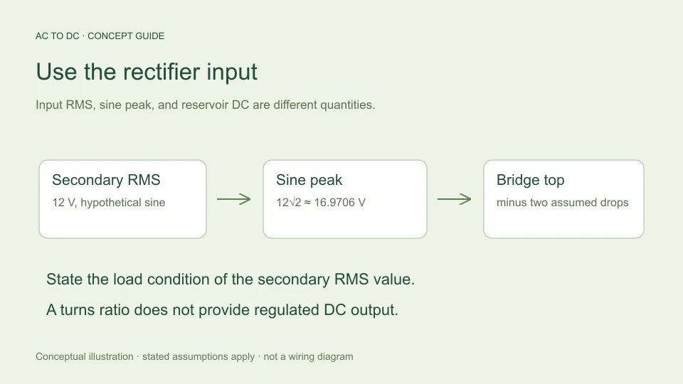
The input to a rectifier calculator is the voltage actually applied to the rectifier, expressed using the convention the model expects. When a bridge is supplied from a transformer secondary, that generally means the secondary voltage, not the primary voltage and not a desired DC output written elsewhere in the system.

This may sound obvious, but many apparent conversion errors start with a correctly entered number that describes the wrong quantity. A secondary RMS rating, an unloaded reading, a sine-wave peak, and an average rectified output are different descriptions. Understanding where each number belongs is more valuable than memorizing a multiplier without its conditions. This guide explains the distinctions through hypothetical low-voltage examples rather than construction instructions.

Identify the node before choosing the number

Imagine a block diagram containing an AC source, transformer, bridge, capacitor, and load. Each boundary can have a different voltage waveform. A model of the bridge needs the AC waveform at its input terminals. A model of a downstream regulator instead needs the regulator’s own input and output conditions.

If the rectifier is connected to a secondary described as 12 V RMS under specified conditions, enter that secondary value when those conditions match the calculation. Entering a primary-side voltage into the same bridge model would describe a different circuit. Entering a target regulated output would also be a category error because it is an intended result after additional circuitry, not the bridge’s AC input.

Write a short label beside your value: “secondary, sinusoidal RMS, stated load condition.” That label preserves information a bare number cannot carry.

RMS is a waveform property

For a periodic waveform v(t), RMS is the square root of its mean squared value over one period. A sinusoid can be written v(t) = Vm sin(ωt). Squaring gives Vm² sin²(ωt). The mean of sin² over a complete cycle is one half, so the resulting RMS voltage is Vm/√2.

Rearranging gives Vm = √2 Vrms. Thus a 12 V RMS sine has an ideal crest of approximately 16.9706 V. This step is a mathematical statement about the sine waveform, not an assertion that a transformer produces perfectly fixed voltage under every load.

The relation also does not convert every possible AC waveform. A number reported as RMS can describe a non-sinusoidal signal, for which the same square-root-of-two peak relationship need not hold. The calculator explicitly restricts its model to sinusoidal input.

A transformer ratio is not a regulator

An ideal turns-ratio model scales primary and secondary voltage together. It does not hold the secondary constant while the primary changes. Real transformers also have impedance that influences the output under load.

Hammond Power Solutions’ voltage-regulation explanation defines regulation using the difference between no-load and full-load secondary voltage relative to the full-load value. This is a description of transformer behavior, not the same function as an electronic regulated DC supply.

The distinction matters because an unloaded secondary measurement need not match a loaded rating exactly. A rectifier estimate made from one condition should not silently be compared with a measurement from another. Record the operating condition and use the value appropriate to the question being asked.

Work through an illustrative regulation calculation

Suppose a hypothetical transformer has 12 V RMS at the specified full-load condition and 13.2 V RMS at no load. Using the stated convention, the difference is 1.2 V relative to 12 V, or 10%. This is an invented arithmetic example, not a specification for a real transformer.

The corresponding sine peaks would be approximately 16.9706 V and 18.6676 V. If a simplified bridge model subtracts two assumed 0.7 V diode drops, the available top levels become approximately 15.5706 V and 17.2676 V respectively.

These numbers show why the input condition affects a capacitor-filtered estimate. They do not model the complete transition from no load to full load, and they do not establish the voltage rating required for a physical component. That needs justified worst-case conditions and the applicable device specifications, beyond this illustrative comparison.

The filter determines which DC quantity is relevant

An ideal unfiltered full-wave rectifier averages to 2Vm/π, about 0.900316 times sinusoidal RMS input. A reservoir capacitor changes the waveform because it stores charge near the crests and supplies the load between charging intervals.

Consequently, “12 V RMS becomes about 10.8 V average” and “a lightly loaded capacitor can approach the sine peak minus diode drops” are descriptions of different models. Treating them as competing universal rules creates confusion that disappears once the filter and output quantity are named.

Hammond Manufacturing’s rectifier guide distinguishes rectifier and filter arrangements and warns that losses must be considered. The site’s formula guide derives the ideal averages and the separate filtered approximation used by the calculator.

Include load and capacitance for a filtered estimate

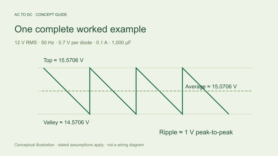
The site’s filtered bridge model estimates ripple from I/(2fC), where I is an approximately constant DC load current, f is the AC input frequency, and C is capacitance in farads. The estimated valley is the available top minus that peak-to-peak ripple. The average is approximated by the midpoint.

With 12 V RMS, 50 Hz, 0.1 A, 1,000 µF, and 0.7 V per diode, ripple is 1 V peak-to-peak. The estimated average is 15.0706 V and valley is 14.5706 V. An RMS input by itself would not provide these results because current and capacitance determine the assumed discharge.

The charge-balance relationship is discussed in TI TIDUB95, section 3.1. Here it is used only within the explicit simplified model, not to promise the performance of unspecified hardware.

Frequency affects the discharge interval

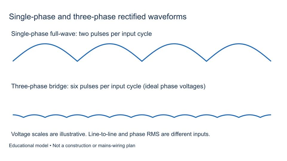
For a full-wave bridge, two crests occur during each input cycle. A 50 Hz input therefore gives 100 Hz ripple repetition in this model, while 60 Hz input gives 120 Hz. The approximate discharge interval changes accordingly.

Keep the calculator’s frequency convention straight: it accepts AC input frequency. If 100 Hz ripple frequency is entered into a field expecting 50 Hz input, the formula applies the factor of two again and underestimates ripple by a factor of two.

Changing frequency in this calculator only changes the modeled interval. It does not validate that a particular transformer or other component is suitable for operation at that frequency. The software’s accepted input range describes its numerical scope, not equipment compatibility.

Voltage alone cannot establish current capacity

Knowing a secondary’s voltage does not reveal its winding-current limit, thermal behavior, available power, or response to capacitor charging pulses. Two sources with the same nominal RMS voltage may behave differently under the same rectifier load.

Likewise, average DC load current is not identical to the transformer’s RMS secondary current in a capacitor-input arrangement. Charging occurs over intervals rather than necessarily flowing as a smooth continuous current. The current waveform matters, and the calculator does not solve that waveform or select a transformer.

A useful calculation record therefore separates voltage estimation from current and thermal qualification. Do not infer that a source can supply an arbitrary load merely because the voltage equation produces a plausible number. A positive result is an arithmetic outcome under assumptions, not evidence of available current.

Compare like conditions when checking a reading

When comparing an estimate with a documented measurement, verify that both refer to the same location, load, input condition, waveform convention, and instrument mode. A peak measurement and an RMS measurement can disagree numerically while both are correct for their respective definitions.

Similarly, a filtered capacitor voltage measured under load should not be compared with an ideal unfiltered average. First reconstruct the intended model. Then identify effects the simplified estimate omits, such as source impedance, nonlinear diode characteristics, capacitor ESR, and transient behavior.

This is a diagnostic reasoning process rather than a procedure for probing equipment. Measurement techniques and safety requirements depend on the actual circuit and instruments. The calculator is designed to explain model relationships, not to replace suitable equipment knowledge or practical verification.

Create a useful input record

For an estimate you want to reproduce later, save the source of the RMS value, its specified load condition, assumed waveform, input frequency, selected rectifier model, and all filtered-load settings. State whether values are nominal, measured, bounded by a specification, or deliberately hypothetical.

For example: “hypothetical 12 V sinusoidal RMS at bridge input, 50 Hz, constant 0.1 A load, 1,000 µF, two fixed 0.7 V diode drops.” That description is compact but contains the information needed to reconstruct the default filtered calculation.

If a different secondary condition is later supplied, update the input record and recalculate rather than silently substituting a new voltage into an old conclusion. This habit keeps the transformer’s role, the rectifier’s role, and the limits of the model visible in the final result.

Treat a sensitivity comparison as a comparison

One useful exercise is to change only the input RMS assumption. If a hypothetical sine input falls from 12 V RMS to 11.4 V RMS while fixed diode drops and discharge settings remain unchanged, the sine peak falls by approximately 0.8485 V. In this simplified model, estimated top, midpoint average, and valley all fall by that same amount because calculated ripple has not changed.

This is a direct consequence of holding current, frequency, and capacitance fixed. A real load may respond to voltage, and a real source may change shape or impedance under a different condition. Those effects are not captured by the controlled comparison. State what was held fixed so another reader can understand the conclusion.

That distinction also makes troubleshooting more efficient. A mathematical sensitivity result answers “what does this model do if this input changes?” It does not answer “what will every physical source do?” Using the first question honestly provides insight without implying the second has been solved.

Filed under rectifier basics component behavior

Topics: transformer voltage · RMS · voltage regulation