Bridge rectifiers at 50 Hz and 60 Hz: what changes?

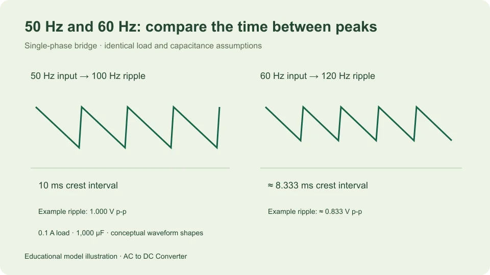
A single-phase full-wave bridge provides two rectified crests during each input cycle. A 50 Hz sinusoidal input therefore produces a repeating full-wave pattern at 100 Hz, while 60 Hz produces 120 Hz. With the same constant load current and capacitance in a simple filter model, the shorter interval at 60 Hz gives a smaller estimated peak-to-peak ripple.

This comparison changes frequency while deliberately holding RMS voltage, waveform shape, diode assumptions, load, and capacitance fixed. It does not predict that arbitrary equipment designed for one supply frequency can operate on another. Transformer behavior, ratings, and control circuits are outside this limited comparison.

Count the events in one input cycle

A sine input completes one full positive-and-negative cycle in a time T = 1/f. At 50 Hz, that is 0.02 seconds, or 20 milliseconds. At 60 Hz, it is approximately 0.016667 seconds, or 16.667 milliseconds.

Full-wave rectification makes both half-cycles contribute positive output. The positive crest from one half-cycle is followed by another rectified crest half an input period later. Their approximate separation is therefore 1/(2f): 10 milliseconds at 50 Hz, and approximately 8.333 milliseconds at 60 Hz.

These time relationships follow from the waveform geometry. They do not depend on choosing a particular smoothing capacitor. A capacitor can change how far the output falls between events, but it does not change the fact that an ideal single-phase bridge receives two crests per input cycle.

Keep input frequency and ripple frequency separate

The calculator’s frequency input is the AC input frequency. In bridge modes it reports ripple frequency as twice that value. Enter 50 for a 50 Hz source; do not enter 100 merely because you expect 100 Hz output ripple.

The distinction matters in the small-ripple formula ΔVpp ≈ I/(2fC). The factor two already accounts for the two bridge charging opportunities. If you enter the doubled ripple frequency for f and retain the factor two, you count the doubling twice and predict half the intended ripple.

Texas Instruments TIDUB95, section 3.1 presents a charge-balance capacitor relation and identifies the full-bridge repetition rate as twice the input frequency. In this article the numerical comparisons are independently worked examples using that stated model.

Calculate a 50 Hz example

Choose an illustrative 12 V RMS sine input, fixed diode drop of 0.7 V per conducting diode, 0.1 A constant load, and 1,000 µF capacitance. The capacitance is 0.001 F. These settings define the example rather than describe a measured supply.

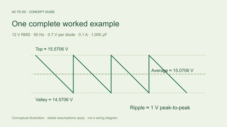
The input peak is 12√2, approximately 16.9706 V. The bridge’s assumed two-diode path reduces the available top to approximately 15.5706 V. At 50 Hz, ripple is estimated as 0.1/(2 × 50 × 0.001), which is 1 V peak-to-peak.

The corresponding modeled valley is top minus ripple, approximately 14.5706 V. Approximating the discharge as linear, its midpoint average is top minus half the ripple, approximately 15.0706 V. Ripple repetition is 100 Hz, with approximately 10 milliseconds between crests.

Change only the frequency to 60 Hz

Keeping every other example input unchanged, the sine peak and fixed-drop top remain the same in this simplified model. The new ripple estimate is 0.1/(2 × 60 × 0.001), approximately 0.833333 V peak-to-peak.

The valley becomes approximately 15.5706 − 0.833333 = 14.7372 V. The midpoint average becomes approximately 15.5706 − 0.416667 = 15.1539 V. Thus the average changes by only about 0.083333 V in this example, while the ripple span changes by about 0.166667 V.

The modest average change is easier to interpret when all quantities are shown together. The example does not say that frequency raised the available sine crest. It says that the modeled capacitor lost less charge between more closely spaced recharge opportunities, so the estimated valley and midpoint moved upward.

Use ratios to understand the change

With current and capacitance fixed, the formula makes ripple inversely proportional to frequency. Therefore ripple at 60 Hz divided by ripple at 50 Hz is 50/60, or 5/6. The 60 Hz estimate is approximately 83.333% of the 50 Hz estimate, a decrease of approximately 16.667% relative to the 50 Hz value.

The reverse wording uses a different percentage base. Going from 60 Hz to 50 Hz multiplies ripple by 60/50, or 1.2. That is a 20% increase relative to the smaller 60 Hz ripple. Both statements are consistent; the reference value changed.

Ratio reasoning is useful because it does not depend on the particular example current or capacitor. Within the same approximation, doubling frequency halves ripple, doubling current doubles ripple, and doubling capacitance halves ripple. Physical circuits may depart from those simple relationships when the model assumptions stop representing their behavior.

Find capacitance for the same modeled ripple

Rearranging the same equation gives C ≈ I/(2fΔVpp). For an illustrative 0.1 A current and target 1 V p-p ripple, the estimate is 0.001 F at 50 Hz, or 1,000 µF. At 60 Hz it becomes approximately 0.000833333 F, or 833.333 µF.

This arithmetic is a comparison of idealized capacitance values, not a component selection. Actual capacitor tolerances, voltage conditions, ripple-current heating, ESR, aging, and application requirements have not been assessed. A target value calculated from charge balance does not establish that a named capacitor is suitable.

For a supply that must satisfy the same ripple target at either frequency under the model, the lower frequency demands more capacitance. That statement is limited to the discharge relationship. Other design constraints can still dominate, and the calculator does not rank them or guarantee a completed supply design.

Compare an unfiltered bridge

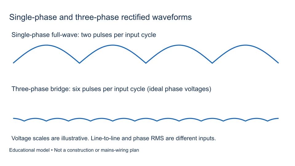
An ideal unfiltered full-wave average is 2Vm/π, where Vm = √2 Vrms. Frequency does not appear in that expression because the normalized waveform shape and its average fraction of peak are unchanged when the cycle is stretched or compressed in time.

At the same 12 V RMS input, ideal full-wave average remains approximately 10.8038 V at both 50 Hz and 60 Hz. Peak remains approximately 16.9706 V, and the valley is zero. What changes is how often the humps repeat: 100 times per second versus 120.

This is why a frequency input can change the reported ripple repetition rate without changing an ideal unfiltered average. Frequency dependence is model-specific. Applying the filtered ripple relationship to an unfiltered waveform, or expecting every output statistic to vary with frequency, confuses different questions.

Contrast half-wave timing

An ideal half-wave rectifier has one contributing crest per input cycle, followed by the blocked half-cycle. Its waveform repeats at the input frequency: 50 Hz for a 50 Hz source, or 60 Hz for a 60 Hz source. Its ideal complete-cycle average remains Vm/π for the same input RMS and sine shape.

The main calculator does not offer a half-wave capacitor-filtered model. Do not take its bridge filter settings and assume the same factor-two timing applies to another circuit. A half-wave smoothing model would need to state its own recharge interval and assumptions explicitly.

Recognizing the event count is a useful general habit. First identify the actual rectifier configuration and waveform, then count the relevant repeat events. Only afterward choose a formula that uses input frequency or ripple frequency consistently.

Write a comparison that another reader can reproduce

A concise comparison should state what stayed fixed as carefully as what changed. For these examples, write “12 V RMS sine at the bridge input, 0.7 V assumed per diode, 0.1 A constant load, and 1,000 µF; compare 50 Hz with 60 Hz.” Then give ripple frequency, peak-to-peak ripple, average, and valley under the same approximation.

Avoid a statement such as “60 Hz produces more DC” without those conditions. It hides whether the input RMS changed, whether a capacitor was present, and whether DC means peak or average. A reader cannot reproduce that claim, and a different circuit could make it misleading.

If you want to study two variables, make two separate comparisons first. For instance, change frequency with current fixed, then change current with frequency fixed. After those effects are understood, calculate the combined case. This keeps a smaller ripple caused by a higher frequency from being confused with a smaller ripple caused by a lighter load. The discipline is useful even when a calculator can update all fields at once: a clean question produces a result that is easier to interpret and check.

Round after the comparison

For a small difference between modeled averages, retain sufficient intermediate digits before rounding the final values. In the example, rounding both averages immediately to 15 V would hide the change caused by frequency, even though the ripple estimates remain different. On the other hand, displaying many digits does not establish that a physical supply behaves to that precision.

A useful presentation gives approximately 15.071 V versus 15.154 V average, with 1.000 V versus 0.833 V p-p ripple, and labels both as estimates under unchanged assumptions. The arithmetic detail supports the comparison without turning it into a measurement claim.

Recognize the simplified model’s boundary

The filtered bridge calculation assumes approximately constant current, negligible recharge time, and a roughly linear small discharge. It rejects estimated ripple above 20% of the available top. That threshold is a tool guardrail chosen to limit the approximation’s scope, not a guaranteed accuracy boundary.

The source and rectifier can respond to frequency in ways omitted here. Transformer regulation and impedance, diode conduction, capacitor ESR, and changing load may alter the real waveform and its top. Holding those effects fixed in an example is useful for isolating one mathematical relationship, but does not make them disappear from hardware.

Use the AC to DC calculator to reproduce both frequency cases and compare all reported values. The capacitor ripple guide explains the charge-balance assumption in more detail. Keep the input convention, circuit, and operating conditions beside the answer so a 50 Hz versus 60 Hz comparison remains specific and meaningful.

Filed under worked examples rectifier basics

Topics: 50 Hz · 60 Hz · bridge rectifier · ripple frequency