Smoothing capacitor calculation: from load current to ripple

A smoothing capacitor calculation answers a particular question: how much charge storage would produce a chosen voltage change during an assumed discharge interval? It does not, by itself, choose a suitable capacitor or establish the output of every AC power supply. Keeping that distinction clear makes the arithmetic much more useful.

This guide considers a single-phase bridge rectifier supplied by sinusoidal AC. The simplified load draws approximately constant current. The capacitor is assumed to recharge near each rectified crest, then discharge almost linearly between crests. These assumptions lead to a convenient estimate that can be checked with units and a worked example. They also explain when a more detailed circuit model is needed.

Define the ripple you actually mean

Ripple is the changing part of the output. In this calculation, allowed ripple means peak-to-peak voltage: the difference between the upper and lower capacitor voltage during a steady repeating cycle. A 1 V peak-to-peak allowance does not mean 1 V RMS, and it does not describe a regulator’s output noise.

Write down the quantity before entering a number. For example, a hypothetical requirement might be “no more than 1 V peak-to-peak ripple at the reservoir capacitor under the stated steady load.” That wording identifies both the location and the measurement convention. A requirement for a downstream regulated rail needs a different analysis because the regulator changes how input disturbances reach its output.

The AC to DC calculator reports capacitor ripple as peak-to-peak voltage. Its peak, average, and valley results are separate quantities, rather than alternative names for the same output.

Derive the charge-balance estimate

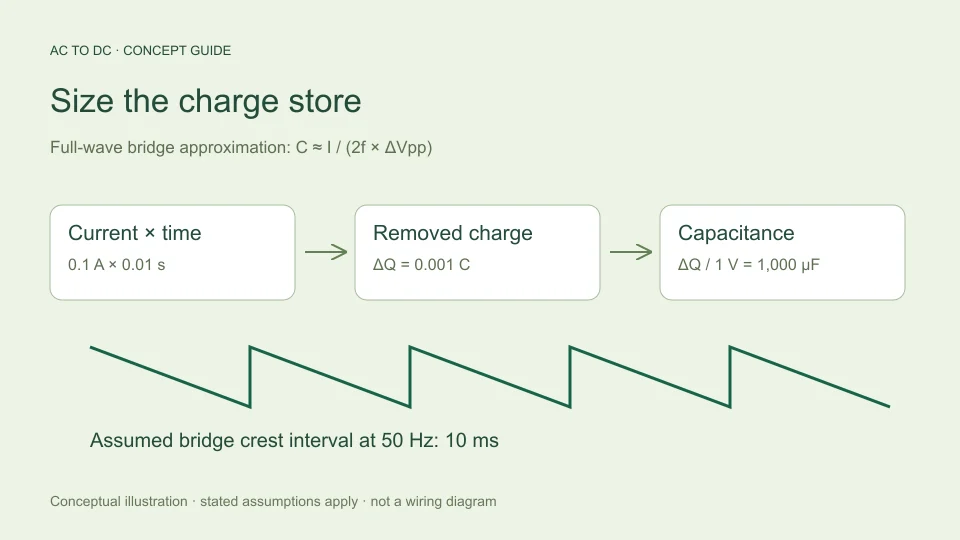
Capacitance relates a change in stored charge to a change in voltage: ΔQ = CΔV. If a constant current I flows for an interval Δt, the removed charge is IΔt. Equating the two expressions gives ΔV = IΔt/C. Rearranging for capacitance gives C = IΔt/ΔV.

A full-wave bridge has two rectified crests in one input cycle. If input frequency is f, the crest-to-crest interval is 1/(2f). Approximating the entire interval as capacitor discharge therefore gives:

C ≈ I/(2fΔVpp).

The charge relation and the distinction between input frequency and doubled bridge ripple frequency are described in Texas Instruments TIDUB95, section 3.1. The remaining calculation here follows directly from rearranging that relationship under the stated assumptions. Actual charging takes time, so the approximation is not a substitute for a simulated or measured waveform.

Keep amperes, hertz, and farads consistent

Use amperes for load current, hertz for the AC input frequency, and volts for allowed peak-to-peak ripple. The resulting capacitance is in farads. To express that answer in microfarads, multiply by one million.

Suppose current is written as 100 mA. Convert it to 0.1 A first. Likewise, 1,000 µF equals 0.001 F. Entering “100” into an amperes field when the intended quantity is 100 mA creates a thousandfold error. Entering “1,000” as farads when the intended value is microfarads creates a millionfold error.

A dimensional check helps: an ampere is a coulomb per second, so current multiplied by time is charge. Dividing charge by volts gives farads. If the expression has leftover seconds or an unexpected unit, revisit the substitutions before interpreting the numerical answer.

Work through a 50 Hz example

Take a hypothetical steady load of 0.1 A, input frequency of 50 Hz, and allowed ripple of 1 V peak-to-peak. The bridge crest interval is 1/(2 × 50) = 0.01 seconds. The assumed charge removed is 0.1 × 0.01 = 0.001 coulombs.

Dividing 0.001 coulombs by the 1 V allowance gives 0.001 F, or 1,000 µF. Checking in the opposite direction gives ripple ≈ 0.1/(2 × 50 × 0.001) = 1 V. This reverse calculation catches an accidentally inverted formula or missed microfarad conversion.

The answer is an estimated capacitance under the model, not a recommendation to install a particular part. A real component has tolerances and operating limits. The circuit also needs checks that this charge-storage equation does not provide, including behavior during startup and the current waveform while the capacitor recharges.

See how frequency and current change the result

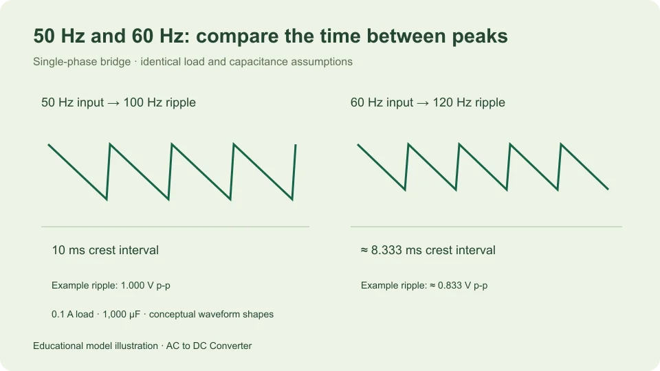
At 60 Hz, keeping the same 0.1 A current and 1 V ripple allowance gives C ≈ 0.1/(120 × 1) = 0.0008333 F, or about 833 µF. The shorter interval between bridge crests reduces the charge that must be stored for each discharge period.

At 50 Hz, doubling current to 0.2 A while preserving the 1 V allowance doubles the estimated capacitance to 2,000 µF. Halving the allowance to 0.5 V doubles it again to 4,000 µF. These proportional relationships follow from the equation and are useful for checking a calculation without reproducing every decimal.

Do not transfer the bridge’s factor of two to a half-wave circuit. A half-wave rectifier has one charging opportunity per input cycle. Under an otherwise comparable discharge approximation, the interval becomes 1/f. The circuit topology must be identified before the frequency multiplier is chosen.

Connect capacitance to peak and valley voltage

Capacitance determines an estimated voltage swing, but that swing needs a starting level. In the site’s filtered bridge model, the available top is approximately √2 times sinusoidal RMS input voltage minus two assumed diode forward drops.

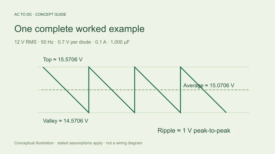
For 12 V RMS and an illustrative 0.7 V drop per diode, the available top is about 15.5706 V. With the 1 V ripple from the previous example, the estimated valley is 14.5706 V. Approximating the discharge as linear places the average halfway between them, about 15.0706 V.

Those figures are internally consistent model outputs. They do not guarantee that a particular transformer, bridge, capacitor, and load will produce those readings. For the reasoning behind the midpoint average and its limitations, see AC to DC formulas. A capacitor changes the waveform; it does not magically create regulated voltage.

Check the approximation before relying on it

The assumed straight discharge line is easiest to interpret when ripple is relatively small compared with the available peak. Large ripple makes the simple picture less representative. The calculator rejects filtered cases where the estimated ripple exceeds 20% of that peak.

This percentage is a tool guardrail, not a physical boundary between valid and invalid circuits, and not a guarantee of a particular percentage error. A case below the guardrail still omits source resistance, conduction angle, diode dynamics, capacitor losses, and changing load behavior. A rejected case needs a more appropriate circuit model rather than an artificial input change designed only to make the warning disappear.

At zero load, the idealized equation gives zero discharge ripple. That is a limiting case of the model. It omits leakage and other currents, so it should not be presented as proof that an actual unloaded output will be perfectly constant.

Separate capacitance from a complete capacitor specification

A value in microfarads describes only one component property. It does not specify voltage capability, ripple-current capability, temperature behavior, life, or construction. Those properties require the actual manufacturer’s data and the circuit’s operating conditions.

TDK’s aluminum electrolytic capacitor technical information explains that ripple-current heating and operating temperature affect useful life. That is a different question from the charge-balance calculation above. Increasing nominal capacitance alone does not establish that every other component limit has been satisfied.

It is therefore helpful to label your result “estimated capacitance for the stated ripple target,” then keep a separate list of verification tasks. This preserves the value of a quick calculation without allowing it to stand in for component qualification, thermal analysis, or practical circuit validation.

Record a reproducible calculation

Save the circuit model, input frequency, load-current assumption, allowed ripple convention, unit conversions, and final capacitance estimate together. If input RMS voltage and diode drops were used to check peak and valley, record those as well.

For the example here, a clear note is: “single-phase full-wave bridge, 50 Hz input, constant 0.1 A load, approximately 1 V peak-to-peak reservoir ripple; charge-balance estimate C ≈ 1,000 µF.” That statement is far more informative than an isolated capacitor number.

When a measured result differs, compare assumptions before blaming arithmetic. Was current constant? Was frequency the input frequency or ripple frequency? Was the capacitance effective under the test conditions? Was the voltage measured at the same node? A disciplined record turns the calculator into an explanation that can be checked, corrected, and reused appropriately.

Distinguish a nominal value from a worst-case check

The equation can be evaluated with more than one set of assumptions. For example, if a hypothetical effective capacitance were 800 µF rather than the nominal 1,000 µF, the same 0.1 A and 50 Hz model would give 1.25 V peak-to-peak ripple. This is simply a sensitivity example; it does not assign a tolerance to any real component.

Similarly, a hypothetical increase in load to 0.12 A would produce 1.5 V ripple with 800 µF. That result follows from combining the changed assumptions explicitly. It is more informative than rounding the nominal answer upward and assuming that every uncertainty has been covered. A worst-case study needs justified input bounds and a model adequate for the decision being made.

The important habit is to preserve the reason for each value. Distinguish a measured capacitance, a data-sheet limit, a nominal marking, and a deliberately hypothetical test value. Each can belong in a calculation, but they support different conclusions. A transparent estimate shows both the arithmetic and the provenance of the inputs, allowing another reader to check the result without guessing which conditions were intended.

Filed under capacitor filtering worked examples

Topics: smoothing capacitor · ripple voltage · charge balance