AC/DC Calc
power supply concepts · worked examples
Why AC to DC output voltage varies with line, load, and components
Use controlled comparisons to distinguish arithmetic changes from effects outside a simplified rectifier model.
A filtered rectifier output is not generally one immutable number attached to an AC voltage label. Its waveform can change when the source, load, or component behavior changes. A calculator can explain some of those dependencies, but only the dependencies represented in its equations.
The useful approach is to separate controlled model comparisons from predictions about complete hardware. In a controlled comparison, one input changes while the others are deliberately held fixed. In a real circuit, several quantities may move together. Understanding that distinction helps explain why a calculation and a measurement can differ without either difference being a simple arithmetic mistake. This guide works through the variables in the site’s filtered bridge estimate.
Start with a complete baseline
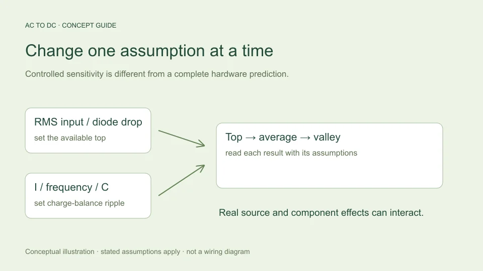
Use a baseline that includes more than RMS voltage. The default filtered bridge example is 12 V sinusoidal RMS at the rectifier input, 50 Hz AC input frequency, an assumed 0.7 V forward drop per diode, constant 0.1 A load, and 1,000 µF capacitance.
The model’s available top is approximately 12√2 − 1.4 = 15.5706 V. Its charge-balance ripple is 0.1/(2 × 50 × 0.001) = 1 V peak-to-peak. The estimated midpoint average is 15.0706 V and the valley is 14.5706 V.
These values establish a reproducible reference. Without the model, load, frequency, and capacitance, saying “12 V AC produces this DC voltage” leaves out information that materially affects the result. Record whether each input is measured, nominal, specified, or deliberately hypothetical.
Change RMS input while holding the other assumptions fixed
Within the selected model, top voltage is √2 times RMS input minus two fixed diode drops. A change of 1 V RMS therefore changes the modeled top by approximately 1.4142 V, provided the result remains above the diode threshold.
For a hypothetical fall from 12 V RMS to 11.4 V RMS, the top falls by about 0.8485 V. Because current, frequency, and capacitance were held fixed, estimated ripple remains 1 V. The modeled average becomes about 14.2220 V and the valley about 13.7220 V.
This is a sensitivity calculation, not a universal prediction of how a source responds to changed conditions. If the load is voltage-dependent or the source waveform changes, holding the other inputs fixed may not represent the physical case. State that limitation rather than silently interpreting the comparison as equipment performance.
Separate source variation from transformer regulation
A transformer’s secondary can change with loading as well as with its input. These are related to the source presented to the rectifier but are not the same question as the bridge’s own mathematical conversion.
Hammond Power Solutions’ regulation explanation relates no-load and full-load secondary voltage through transformer impedance. The important consequence for a calculator is that the correct RMS input must correspond to the operating condition being evaluated.
If one calculation uses an unloaded secondary reading and another uses a loaded value, their outputs can differ because their inputs describe different conditions. A clean comparison identifies that change explicitly. The calculator does not infer a transformer regulation curve from one nominal voltage or solve the source impedance during capacitor charging.
Change the assumed diode forward voltage
The filtered bridge model subtracts two forward drops. If each assumed drop increases from 0.7 V to a hypothetical 0.8 V while all other inputs remain fixed, the available top decreases by 0.2 V. Estimated average and valley decrease by the same 0.2 V because the charge-balance ripple calculation is unchanged.
This mathematical comparison does not imply that real forward voltage is an independent knob unaffected by operating conditions. Toshiba’s rectifier-diode explanation notes that the forward characteristic depends on current and temperature.
The calculator uses a fixed value so the approximation is explicit and reproducible. A more detailed device model can allow voltage and current to interact throughout the waveform. The fixed-drop result should be reported as an estimate under an assumption, not a claim that every bridge always loses a particular voltage.
Increase load current in the charge-balance model
With I/(2fC), doubling current doubles estimated peak-to-peak ripple when frequency and capacitance remain fixed. In the baseline example, changing load from 0.1 A to 0.2 A increases ripple from 1 V to 2 V.
The assumed top remains 15.5706 V in this isolated comparison. Average falls to approximately 14.5706 V because half of the 2 V ripple is subtracted. Valley falls to approximately 13.5706 V because the entire ripple is subtracted. Peak, midpoint, and minimum therefore do not all respond in the same way to this particular model change.
Real source impedance and current-dependent diode behavior can also change the top under heavier loading. The simplified model omits those effects. That is why the controlled comparison explains one mechanism without claiming to calculate every reason a loaded output might fall.
Distinguish constant-current and resistive loads
A constant-current assumption means the model holds load current fixed as voltage changes. A resistive load instead follows current equal to voltage divided by resistance, so its current changes during the ripple cycle.
For example, a hypothetical resistance carrying 0.1 A at 15 V would be 150 Ω. At a different instantaneous voltage, the same resistance would not necessarily draw exactly 0.1 A. Reusing one average-current number can still be a useful approximation in a limited study, but its meaning should remain visible.
The site’s filtered mode does not accept resistance or solve exponential discharge through a resistor. Its ideal unfiltered modes have a different stated load assumption. Similar labels should not obscure that the models answer different questions. Identify the load type before deciding whether a calculator result fits the intended situation.
Change capacitance and preserve its units
At the baseline current and frequency, increasing capacitance from 1,000 µF to 2,000 µF halves the charge-storage ripple from 1 V to 0.5 V. The estimated average becomes 15.3206 V and the valley 15.0706 V. The modeled available top remains unchanged.
Reducing effective capacitance to a hypothetical 800 µF instead gives 1.25 V ripple, an average near 14.9456 V, and a valley near 14.3206 V. This is an illustrative parameter change, not an assigned tolerance for an unspecified component.
Capacitance is entered in microfarads and converted to farads for the equation. A unit mistake can dominate all of the subtle effects under discussion. Check the conversion before attributing a surprising result to a complicated circuit phenomenon.
Change frequency without double-counting the bridge
A full-wave bridge provides two charging opportunities per AC input period. The approximate discharge interval is therefore 1/(2f), where f is the input frequency. A change from 50 Hz to 60 Hz with other assumptions fixed reduces baseline ripple from 1 V to about 0.8333 V.
The charge-balance relation and doubled bridge ripple frequency are described in TI TIDUB95, section 3.1. Keep the convention clear: 100 Hz is the modeled ripple repetition for a 50 Hz input, not the value to enter into a field already labeled AC input frequency.
This comparison does not determine frequency suitability of a real transformer or other hardware. It only changes the interval in the reservoir model. The equipment question needs its own specifications and analysis.
Recognize effects the input fields do not represent
The calculator does not include capacitor ESR, leakage, source resistance, charging conduction angle, diode dynamics, startup inrush, load transients, or a downstream regulator. Changing none of the visible inputs does not imply that these effects are absent from a real circuit.
For instance, ESR can contribute a current-related voltage component in addition to charge-storage ripple. A regulator can respond to reservoir variation according to its own operating conditions and control behavior. These mechanisms cannot be reconstructed from the displayed average alone.
A useful interpretation therefore has two parts: “the model predicts this under these inputs,” followed by “these other effects remain outside the model.” That statement is more precise than claiming every observed variation must be caused by one input or that the calculated value is guaranteed to match hardware.
Use the small-ripple guardrail honestly
The site rejects filtered estimates whose calculated ripple exceeds 20% of available peak. That is a chosen limit on the simplified approximation, not a manufacturer rating, a universal physical threshold, or a claim that every accepted result has a fixed error percentage.
If an input change triggers rejection, the result is useful information about scope. Do not change an unrelated setting merely to make the warning disappear. Either evaluate a genuinely different scenario or use a more appropriate circuit model.
For accepted cases, the same discipline still applies. Passing the guardrail does not verify component ratings, thermal behavior, regulation, or safety. It simply allows the calculator to present the selected small-ripple estimate under its documented assumptions.
Compare scenarios one change at a time
Create a baseline record, change one justified input, and compare top, average, valley, and ripple together. If several real conditions change simultaneously, list them rather than pretending one controlled sensitivity explains the whole observation.
For an independent check, derive the difference directly where possible. Doubling capacitance halves charge-storage ripple; adding 0.1 V to each of two assumed diode drops lowers the modeled top by 0.2 V. These relationships help catch data-entry errors before detailed interpretation.
Finally, retain the question the calculation answered. A sensitivity study explains dependencies within a model. A prediction about a particular power supply requires its actual circuit, operating conditions, specifications, and verification. Keeping those purposes distinct makes each numerical result more useful and easier to assess.
Filed under power supply concepts worked examples