AC/DC Calc
rectifier basics
Full-Wave Bridge Rectifiers: Output Waveform, Average, and Filtering
Understand what a bridge changes, why two diode drops appear, and how its ideal average differs from a capacitor-filtered estimate.
A full-wave bridge rectifier uses both half-cycles of an alternating input to produce one output polarity. That description explains rectification, but it does not by itself establish a smooth output, a fixed DC voltage, or the current a supply can deliver. Those questions require additional assumptions about filtering, load, and source behavior.
For calculation, separate the ideal rectified waveform from the behavior of a capacitor-filtered bridge. The AC to DC calculator provides both an ideal full-wave average and a simplified filtered estimate. Understanding the distinction prevents the common mistake of treating an unfiltered multiplier and a peak-based filtered model as though they describe the same circuit.
What full-wave rectification changes
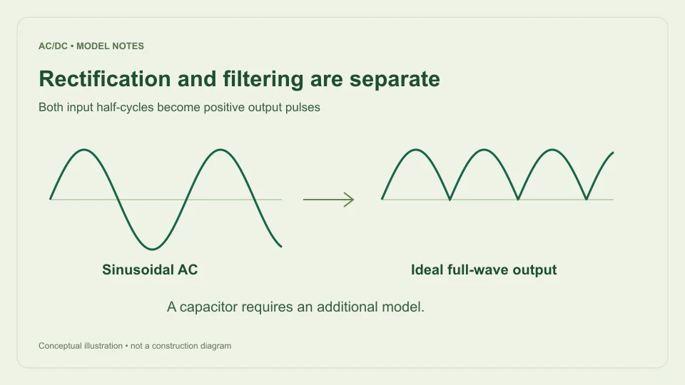
Represent a sinusoidal input by v = Vm sin θ. It is positive during one half of the cycle and negative during the other. An ideal full-wave rectifier delivers the absolute value, Vm|sin θ|, to its output. Both input half-cycles therefore contribute positive output voltage.
The transformation changes polarity behavior without increasing the original sine’s ideal crest. The output peak remains Vm. Between adjacent crests, the ideal unfiltered output reaches zero. Its shape is a sequence of positive half-sines rather than a horizontal DC line.
The Hammond Manufacturing rectifier guide distinguishes bridge arrangements with resistive, capacitor-input, and choke-input loading. Its AC voltage convention is RMS, and it cautions that losses such as diode drop are separate from its simplified guide factors. That separation is useful when deciding which model a calculation should use.
Why a bridge has two conducting drops
A bridge arrangement directs current through a pair of diodes for each conducting input half-cycle. When the input polarity reverses, the other pair provides the corresponding output direction. Under a fixed-forward-drop approximation, the active path therefore contains two assumed diode drops.
For a capacitor-filtered estimate, this leads to Vtop ≈ √2 Vrms − 2Vf, where Vf is the assumed drop of one diode. A setting of 0.7 V means an assumed pair loss of 1.4 V. It does not mean each bridge always loses exactly 1.4 V under every condition.
The calculator does not attempt to reconstruct a device’s current-voltage curve from that single setting. Actual forward behavior varies with operating conditions and device characteristics. The fixed-drop input is a modeling choice that must be recorded with the result. The diode-drop guide explains why a convenient default should not be mistaken for a universal component specification.
Derive the ideal unfiltered average
The average of Vm|sin θ| over a complete cycle is the area under the waveform divided by 2π. There are two identical positive half-sines, each with area 2Vm. Total area is 4Vm, so the mean is 2Vm/π.
For a sine, Vm = √2 Vrms. Substitution gives Vavg = 2√2 Vrms/π, approximately 0.900316 Vrms. With 12 V RMS input, the ideal average is approximately 10.8038 V. The peak is approximately 16.9706 V and the valley is zero.
This result assumes zero diode drop, no smoothing capacitor, and a resistive load. It is not a loaded capacitor-input supply estimate. In particular, its average should not be used as a prediction of the capacitor’s crest level. The full-wave calculator labels the result as an ideal waveform average so that the mathematical meaning stays visible.
RMS, average, and peak remain distinct
Full-wave rectification changes the sign of negative values, but squaring the rectified values produces the same squares as the original sine. The ideal full-wave output RMS is therefore equal to the input RMS. Its average is lower than RMS, while its peak is higher.
For the 12 V RMS example, ideal output RMS is 12 V, average is about 10.8038 V, and peak is about 16.9706 V. These are not conflicting answers. RMS describes the mean-square quantity, average describes the waveform’s mean, and peak describes its largest instantaneous value.
This difference matters when copying a number into another calculation. A bare “10.8 V” label can hide whether the value is an average, RMS, or peak. Report the convention and whether the waveform is filtered. A result that is clear at the point of calculation should remain clear when it appears in a worksheet, article, or design note later.
Why ripple repeats at twice the input frequency
A full input sine cycle contains one positive crest and one negative crest. Full-wave rectification brings both to positive output polarity. Consequently, the output pattern repeats every half input cycle, producing a ripple repetition frequency of 2f.
At 50 Hz AC input, the ideal rectified crests are 10 ms apart and ripple repetition is 100 Hz. At 60 Hz, the spacing is approximately 8.333 ms and repetition is 120 Hz. Frequency describes the timing of the pulses, not their voltage amplitude.
Adding a capacitor does not remove the underlying two charging opportunities per AC cycle in this model. Instead, it changes the waveform between them. The ripple-frequency guide separates this timing relationship from peak-to-peak ripple magnitude and from the harmonic components of a real measured waveform.
What a smoothing capacitor changes
With a capacitor across the output and a load drawing current, the output can remain above the falling rectified input for part of each interval. The capacitor supplies charge during that time, then is replenished near a later crest. The output no longer follows each half-sine down to zero under the small-ripple conditions assumed here.
For a simplified constant-current load, lost charge between crests is approximately I/(2f). Dividing by C gives ripple ΔVpp ≈ I/(2fC). Treating that discharge as approximately linear gives Vavg ≈ Vtop − ΔVpp/2 and Vvalley ≈ Vtop − ΔVpp.
This is a separate waveform model, not a correction applied to the ideal full-wave average. Its average can be nearer the available crest because the capacitor supports the output between crests. The capacitor-ripple article derives the charge relationship and shows how to convert microfarads to farads before using it.
Compare both models with the same AC input
Use 12 V RMS at 50 Hz. In ideal unfiltered full-wave mode, the calculated average is approximately 10.8038 V, the peak is 16.9706 V, the valley is zero, and the ripple repetition frequency is 100 Hz. Peak-to-peak waveform variation is the entire 16.9706 V from zero to crest.
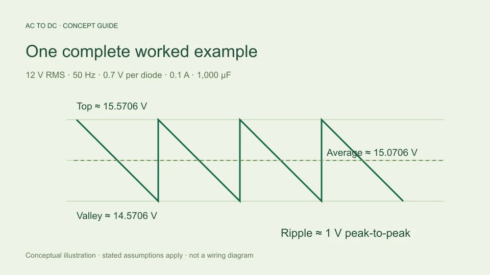
Now specify the filtered bridge model with 0.7 V per diode, 0.1 A constant load, and 1,000 µF. Available top is about 15.5706 V. The approximate ripple is 0.1/(100 × 0.001) = 1 V p-p. Estimated average is about 15.0706 V and estimated valley is 14.5706 V.
The filtered average is higher despite the modeled diode drops because a different output waveform is being averaged. Comparing only the two average numbers can obscure that reason. Listing peak, valley, ripple, and assumptions makes the physical distinction visible and discourages the idea that one of the two equations must simply be wrong.
Know when the simplified bridge estimate is insufficient
The filtered calculator assumes a sinusoidal source, fixed diode drops, approximately constant load current, and small approximately linear ripple. It excludes source impedance, transformer regulation, diode dynamics, capacitor ESR and tolerance, inrush, and regulator behavior. These omissions become relevant when a more faithful waveform prediction is needed.
The tool rejects filtered estimates above a 20% ripple-to-top ratio. That is an application guardrail, not a manufacturer rating or an accuracy certificate. An accepted result can still differ from a real circuit because the selected inputs and assumptions do not capture every physical effect.
The model also does not derive available output current from input voltage. A voltage calculation cannot establish transformer current capability, thermal limits, charging-current stress, or component suitability. Keep the task narrow: it estimates selected voltage quantities under stated assumptions. Equipment choices and practical implementation need appropriate specifications, measurements, and assessment beyond this calculation.
Keep a useful record of the result
A reproducible bridge calculation includes the input RMS voltage at the rectifier terminals, input frequency, whether filtering is included, the output quantity, and every active model setting. For filtered mode, record per-diode drop, assumed load current, capacitance, estimated ripple, and estimated valley alongside average DC.
If another result differs, compare those definitions first. One calculation may be using an ideal unfiltered average while another estimates a capacitor crest. One may enter the primary voltage while another uses the secondary. One may label a peak reading as RMS. These differences can be much larger than rounding effects.
The most useful bridge calculator is therefore one that makes its model visible. A clearly labeled approximation can explain a result and reveal its limits. An unexplained multiplier may produce a neat number while leaving the central circuit question unanswered.
Read a normalized waveform before using actual volts
A normalized plot uses an input peak of one. The ideal full-wave crest is then one, its valley is zero, its average is 2/π, and its RMS is 1/√2. These ratios are easier to compare because they separate waveform shape from amplitude. Multiplying every vertical value by the actual sine peak restores the voltage scale.
For example, multiplying the normalized average 2/π by 16.9706 V gives approximately 10.8038 V. Multiplying the normalized RMS 1/√2 by the same peak gives 12 V. The exercise shows that average and RMS are different summaries of one waveform rather than competing estimates of one unspecified quantity.
A filtered waveform needs its own normalized shape because its lower portion is supported by the capacitor. Drawing an average line across an unfiltered waveform and then labeling it as a capacitor level does not change the underlying model. When reading an illustration, check the axes, the baseline, and whether a capacitor is actually part of the stated circuit. A clear diagram should distinguish waveform transformation from filtering rather than hiding both in a generic “DC” line.
Filed under rectifier basics